A System for Video Surveillance and Monitoring

1 Introduction

• Project Thrust: Cooperative multi-sensor surveillance to support battlefield awareness (DARPA VSAM program [17]).
• Goal (IFD Contract): Develop automated video understanding technology enabling a single human operator to monitor activities over a complex area using a distributed network of active video sensors. Automatically collect and disseminate real-time information to improve situational awareness.
• Military/LE Applications:
  • Perimeter security for troops.
  • Monitoring peace treaties or refugee movements (UAVs).
  • Security for embassies or airports.
  • Stakeouts (collecting time-stamped images of entries/exits).
• Commercial Relevance:
  • Video cameras are cheap, but human monitoring is expensive.
  • Current commercial systems often just record; post-event analysis is too late.
  • Need for continuous (24-hour) monitoring and real-time analysis to alert security during incidents (e.g., burglary in progress, suspicious loitering).
• Core Challenge: Keeping track of people, vehicles, and their interactions in complex urban or battlefield environments.
• VSAM Technology Role:
  • Automatically “parse” people and vehicles from raw video.
  • Determine their geolocations.
  • Insert them into a dynamic scene visualization.
• Developed Capabilities:
  • Robust moving object detection and tracking (temporal differencing, template tracking).
  • Semantic classification (human, human group, car, truck) using shape and color analysis; used to improve tracking via temporal consistency.
  • Human activity classification (walking, running).
  • Geolocation determination:
    • Wide-baseline stereo (overlapping views).
    • Viewing ray intersection with a terrain model (monocular views).
  • Higher-level tracking: Tasking multiple PTZ sensors to cooperatively track objects.
  • System Integration: Transmission of symbolic data packets to a central operator control unit (OCU).
  • Visualization: Graphical user interface (GUI) providing a broad overview of scene activities.
• Demonstration: Yearly demos using a testbed system on the CMU campus.
• Report Scope: Final report for the three-year VSAM IFD program. Emphasizes recent/unpublished results, summarizes older work with references.

2 VSAM Testbed System

• Purpose: Demonstrate how automated video understanding technologies can combine into a coherent system enabling a single operator to monitor a wide area.
• Architecture: Multiple sensors distributed across CMU campus, connected to a control room in the Planetary Robotics Building (PRB).
• Key Components:
  • Sensor Processing Units (SPUs): Remote units processing video from sensors.
  • Central Operator Control Unit (OCU): Integrates symbolic information from SPUs with a 3D site model.
  • Graphical User Interface (GUI): Presents results to the user on a map-based display.

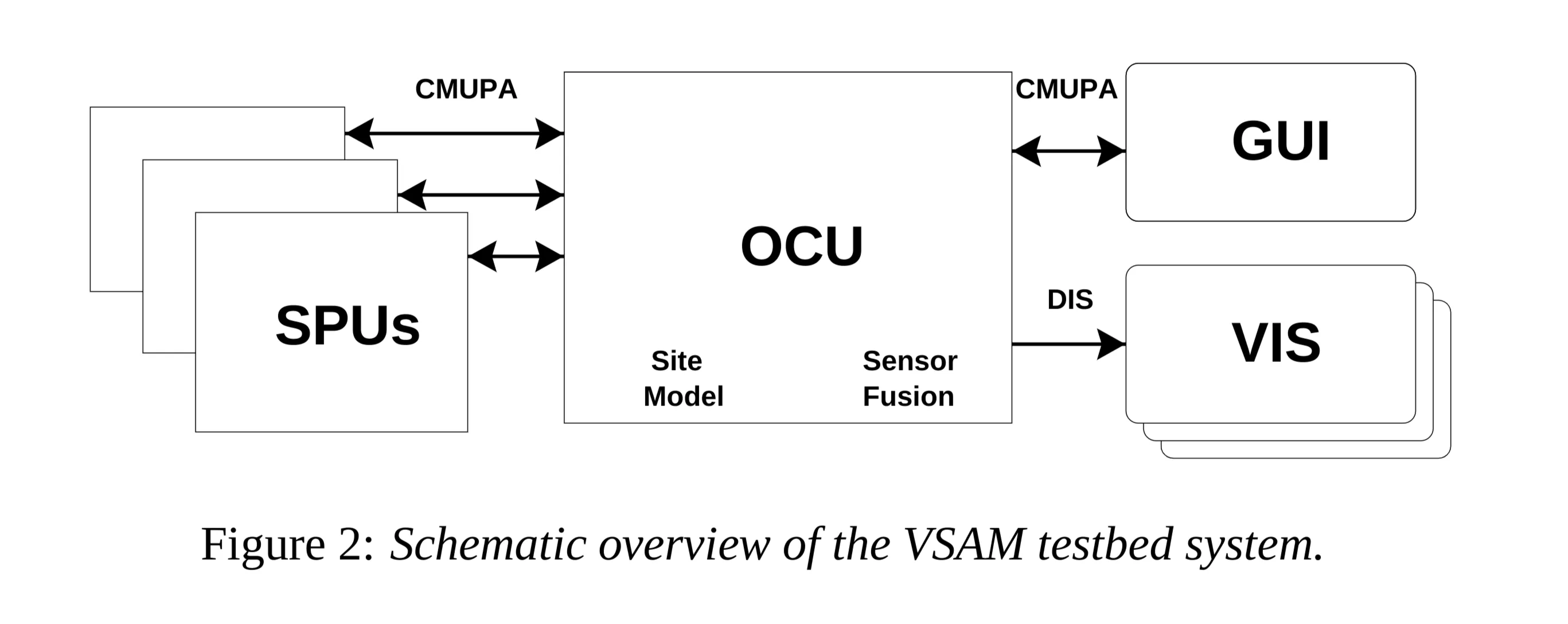
2.1 Sensor Processing Units (SPUs)

• Function: Act as an intelligent filter between a camera and the VSAM network.
  • Analyze video imagery for significant entities or events.
  • Transmit symbolic information (not full video) to the OCU.
• Benefits: Allows seamless integration of different sensor modalities; reduces network bandwidth requirements.
• Sensor Types Handled (Figure 3):
  • Color CCD cameras with active Pan, Tilt, Zoom (PTZ) control.
  • Fixed field-of-view monochromatic low-light cameras.
  • Thermal sensors.
• Logical Structure: Each SPU combines a camera with a local processing computer.
  • Practical Implementation: Most video signals sent via fiber optic to computers located in the central control room rack (Fig 1b).
• Mobile/Special SPUs:
  • Van-mounted relocatable SPU: On-board computing, wireless Ethernet link. Research Issue: Rapid calibration of sensor pose after redeployment for geolocation.
  • SUO portable SPU: (Small Unit Operations)
  • Airborne SPU: (Details below)
  • These require on-board computing power.

2.2 Operator Control Unit (OCU)

• Function: Accepts processed video results (symbolic data) from SPUs, integrates information with a site model and database of known objects to infer activities of interest. Outputs data to GUI/visualization tools.
• 
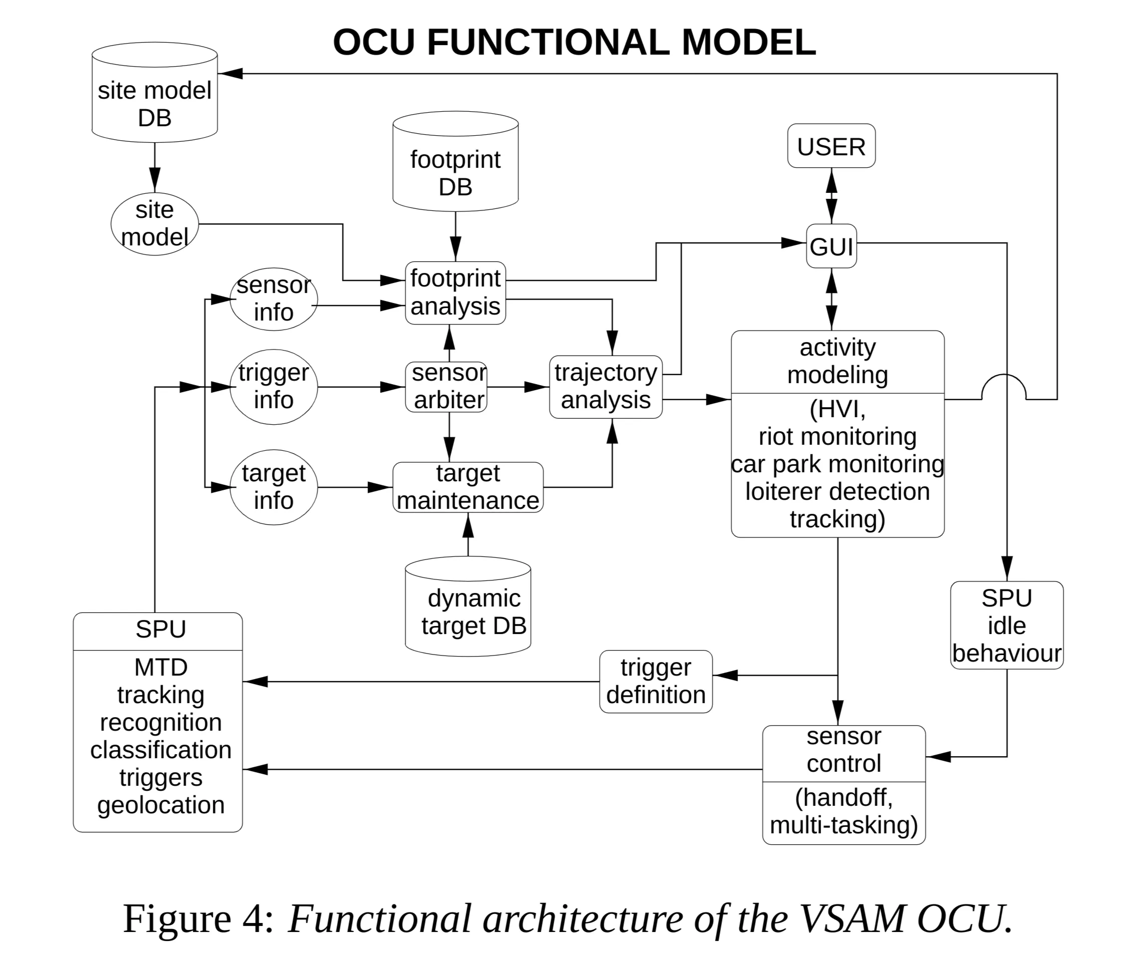
• Key Functionality: Sensor Arbitration:
  • Manages limited sensor assets to avoid underutilization.
  • Allocates sensors to surveillance tasks based on user specifications (track specific objects, watch regions, detect events like loitering).
  • Maintains list of known objects, sensor parameters, and tasks.
  • Uses an arbitration cost function to assign SPUs to tasks.
  • Cost based on: task priority, SPU load, visibility of objects/regions from sensor.
  • Performs greedy optimization to maximize overall system performance.

2.3 Graphical User Interface (GUI)

• Goal: Enable a single human operator to effectively monitor a significant area with multiple targets and interactions, avoiding sensory overload from raw video feeds.
• Approach: Interactive, graphical display using VSAM technology to automatically place dynamic agents (representing people/vehicles) into a synthetic view of the environment.
• Benefits: Visualization is decoupled from original sensor resolution/viewpoint. Significant reduction in transmission bandwidth.
• Figure 5: (a) Operator console (main and portable laptop). (b) Close-up of GUI display screen (map view).
• Features:
  • Map of the area overlaid with:
    • Object locations.
    • Sensor platform locations.
    • Sensor fields of view (FOVs).
  • Optional low-bandwidth, compressed video stream from a selected sensor for real-time display.
• Functionality: Sensor Suite Tasking: Operator tasks individual sensors or the entire suite.
• Control Panel (Lower Left, Tabbed): Organizes controls by entity type (Objects, Sensors, Regions of Interest).
  • Object Controls:
    • Track: Start active tracking of the current object.
    • Stop Tracking: Terminate active tracking tasks.
    • Trajectory: Display trajectory of selected objects.
    • Error: Display geolocation error bounds for object locations/trajectories.
  • Sensor Controls:
    • Show FOV: Display sensor field of view on map (otherwise just position marker).
    • Move: Allow user interaction to control sensor pan/tilt.
    • Request Imagery: Request continuous stream or single image.
    • Stop Imagery: Terminate image stream.
  • ROI Controls (Regions of Interest):
    • Focus sensor resources on specific areas.
    • Create: Interactively define ROI polygon.
    • Specify object types (e.g., human, vehicle) to trigger events within ROI.
    • Specify event types (e.g., enter, pass through, stop in) considered as triggers.

2.4 Communication

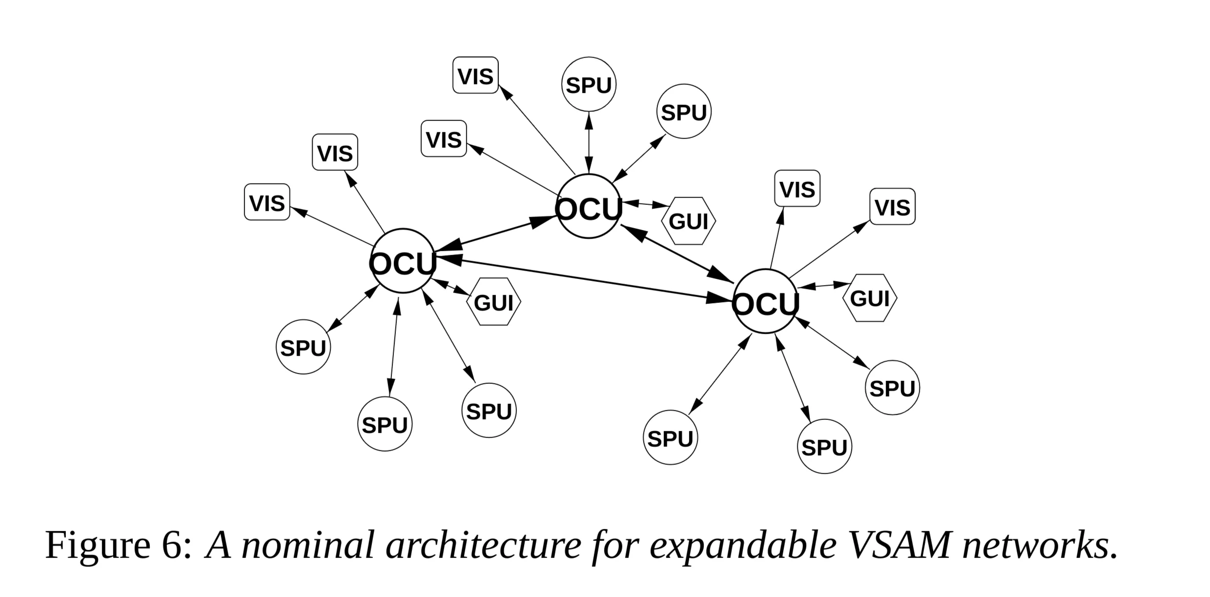
• Network Architecture (Figure 6): Nominally supports multiple OCUs linked together, each controlling multiple SPUs. Each OCU supports one GUI. Output also distributed via Visualization Nodes (VIS).

• 

• Protocols Supported:
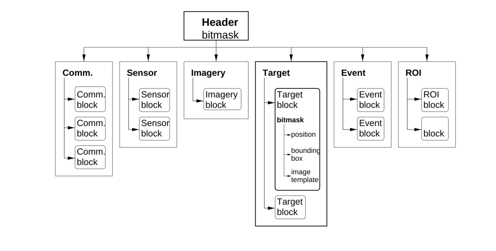
  • CMUPA (Carnegie Mellon University Packet Architecture):
    • Designed for low bandwidth, high flexibility.
    • Compactly packages VSAM information without redundant overhead.
    • Hierarchical decomposition (Figure 7).
    • 6 Data Sections: command, sensor, image, object, event, region of interest.
    • Packet Header: Short bitmask indicates which sections are present.
    • Sections contain multiple data blocks, each potentially with different info layout (described by short bitmasks). Minimizes wasted space.
    • Used for all SPU ←> OCU ←> GUI communication.
    • Specification: http://www.cs.cmu.edu/~vsam (Link may be outdated).
  • DIS (Distributed Interactive Simulation):
    • Used for communication to VIS nodes.
    • Described in detail in [15].
• 
• VIS Nodes:
  • Distribute VSAM output where needed.
  • Provide symbolic representations of activities overlaid on maps or imagery.
  • Unidirectional information flow: OCU → VIS.
  • Uses DIS protocol.
  • Benefit: Easy interface with synthetic environment visualization tools like ModSAF and ModStealth (See Section 4.4).

3 Video Understanding Technologies

• Overall Goal: Automatically “parse” people/vehicles from raw video, determine geolocations, insert into dynamic scene visualization.
• Key Capabilities Developed:
  • Moving Object Detection: Robust routines using temporal differencing and template tracking.
  • Object Classification: Into semantic categories (human, group, car, truck) using shape/color analysis. Labels improve tracking via temporal consistency.
  • Activity Classification: Further classification of human activity (walking, running).
  • Geolocation: Determine 3D locations from image coordinates using wide-baseline stereo or monocular ray/terrain intersection.
  • Higher-Level Tracking: Use geolocations to task multiple PTZ sensors for cooperative tracking.
  • Output: Results displayed on GUI, archived in web-based object/event database.

3.1 Moving Object Detection

• Challenge: A significant and difficult research problem [26]. Detection provides focus for later recognition, classification, activity analysis.
• Conventional Approaches:
  • Temporal Differencing [1]: Very adaptive to dynamic environments, but poor at extracting all relevant feature pixels.
  • Background Subtraction [13, 29]: Provides most complete feature data, but extremely sensitive to dynamic scene changes (lighting, extraneous events).
  • Optical Flow [3]: Can detect independently moving objects with camera motion, but most methods computationally complex (often require specialized hardware for real-time full-frame).
• VSAM Developed Methods:
  • 1. Hybrid Adaptive BGS + 3-frame Differencing (3.1.1): Fast, surprisingly effective. Primary algorithm for most SPUs. Works for static cameras or “step-and-stare” PTZ.
  • 2. Temporal Object Layers (3.1.2): Handles objects stopping, being occluded, resuming motion. Also for static/step-and-stare cameras.
  • 3. BGS from Continuously Panning/Tilting Camera (3.1.3): Extension using clever image evidence accumulation. Real-time on conventional PC.
  • 4. Airborne Platform MTD (Section 3.6): Uses image stabilization (special hardware) + MTD techniques.

3.1.1 A Hybrid Algorithm for Moving Object Detection

• Figure 9: Illustrates problems with standard methods. (a) Background subtraction leaves “holes” when stationary objects (like parked car) move. (b) Frame differencing doesn’t detect the entire object interior.
• Motivation: Combine adaptive background subtraction [18] with three-frame differencing to overcome limitations of each.
• Process:
  1. Perform three-frame differencing to find regions of legitimate motion.
  2. Use adaptive background subtraction within these regions to extract the entire moving object shape.
• Mathematical Formulation:
  • Let $I_n(x)$ be intensity at pixel $x$ at time $t=n$.
  • Three-frame differencing rule: Pixel $x$ is moving if: $(|I_n(x)-I_{n-1}(x)|>T_n(x))$ AND $(|I_n(x)-I_{n-2}(x)|>T_n(x))$ where $T_n(x)$ is a dynamically updated threshold.
  • Problem: Pixels interior to uniform objects are missed.
  • Solution:
    1. Cluster pixels identified by the 3-frame rule into connected regions.
    2. For each region, define its bounding box $R$.
    3. Apply adaptive background subtraction within $R$.
    4. Let $B_n(x)$ be the background model intensity at pixel $x$.
    5. The filled moving blob $b_n$ is defined as: $b_n=\{x:|I_n(x)-B_n(x)|>T_n(x),x\in R\}$
• Background Model and Threshold Update:
  • $B_n(x)$ and $T_n(x)$ are statistical properties learned over time from non-moving pixels.
  • Initialization: $B_0(x)=I_0(x)$, $T_0(x)=$ preset non-zero value.
  • Update Rules (only for pixels determined to be non-moving):
    • $B_{n+1}(x)=\alpha B_n(x)+(1-\alpha )I_n(x)$
    • $T_{n+1}(x)=\alpha T_n(x)+(1-\alpha )(5\times |I_n(x)-B_n(x)|)$
  • If pixel $x$ is moving at time $n$, $B_{n+1}(x)=B_n(x)$ and $T_{n+1}(x)=T_n(x)$.
  • $\alpha$ is a time constant (learning rate).
  • Interpretation: Updates use an Infinite Impulse Response (IIR) filter. $B_n(x)$ is like a local temporal average. $T_n(x)$ is like $5$ times the local temporal standard deviation of intensity.
• Figure 10: Example result. (a) Original image. (b) Detected motion regions using the hybrid algorithm.

3.1.2 Temporal Layers for Adaptive Background Subtraction

• Motivation: A robust system should handle stopped objects and disambiguate overlapping objects, which traditional methods struggle with. Key observation: Legitimate moving objects cause faster intensity transitions than lighting/weather/diurnal changes.
• Approach: Layered detection based on pixel analysis and region analysis.
  • Pixel Analysis: Determine if a pixel is stationary or transient by observing intensity over time.
  • Region Analysis: Agglomerate pixels into moving and stopped regions, assigning them to layers.
• Figure 11: Conceptual diagram. Shows a pixel transitioning between background (B) and layers (L1, L2) via transient periods (D). Spatially related pixels form moving objects (MO) or stopped objects (SO).
• Figure 12: Architecture. Video stream → Image Buffer → Pixel Analysis (Time Diff, Pixel Diff classify as Motion M, Difference D, Similar S) → Region Analysis (Spatio-temporal clustering) → Layer Management (maintains Background B, Layers L1..Lm) → Output (transient regions = moving target, stationary regions = stopped target). Selective Adaptation updates layers.
• Pixel Intensity Profiles (Figure 13): Characteristic shapes based on events at a pixel location.
  • (a) Object moves through pixel: Step change → instability → step back to background level.
  • (b) Object stops on pixel: Step change → instability → settles to a new stable intensity value.
  • (c) Ambient illumination change: Smooth intensity changes, no large abrupt steps.
• Analysis Requirement: Need to observe pixel behavior for a period after a potential step change to interpret its meaning (passing through vs. stopping). Introduces a time delay ($k$ frames, e.g., $k\approx 1$ second). Decisions made about events at time $t-k$.
• Computed Pixel Measures (at time $t$, $k$ frames in past):
  • Motion Trigger $T$: Max absolute intensity difference between frame $t$ and the 5 preceding frames. Captures abrupt changes. $T=\max \{|I_t-I_{t-j}|,\forall j\in [1,5]\}$
  • Stability Measure $S$: Variance of the intensity profile from time $t$ to the present (over $k+1$ frames). Measures stability after potential trigger. $S=\frac{(k+1){\sum }_{j=0}^{k}I(t+j{)}^2-({\sum }_{j=0}^{k}I(t+j){)}^2}{(k+1)k}$ (Note: PDF formula seems to use $k$ samples from $t$ to $t+k-1$? Let’s re-verify. PDF shows sum $j=0$ to $k$, implying $k+1$ samples. Let’s use that. Denominator is $k(k-1)$ in PDF, which implies $k$ samples. Let’s stick to the PDF’s formula for $S$ despite potential inconsistency): $S=\frac{k{\sum }_{j=0}^{k-1}I(t+j{)}^2-({\sum }_{j=0}^{k-1}I(t+j){)}^2}{k(k-1)}$ (Assuming $k$ samples from $t$ to $t+k-1$)
• Transience Map $M(x)$: State per pixel (background=0, transient=1, stationary=2).
  • Update Logic:

    if ((M(x) == stationary or M(x) == background) AND (T > Threshold))
      M(x) = transient
    else if ((M(x) == transient) AND (S < StabilityThreshold)) {
      if (stabilized intensity value == background intensity)
        M(x) = background
      else
        M(x) = stationary
    }
    // Implicitly: if transient and S >= StabilityThreshold, M(x) remains transient.
    

• Region Clustering: Cluster non-background pixels ($M(x)=1$ or $M(x)=2$) into regions $R_i$ using a nearest neighbor spatial filter (radius $r_c$, tolerant to gaps up to $r_c$).
• Region Analysis Algorithm: Analyze each region $R$ based on the $M$ values of its pixels.
  • If all pixels in $R$ are transient ($M=1$): $R\to$ moving object.
  • If all pixels in $R$ are stationary ($M=2$):
    • Remove pixels already assigned to existing layers $L(0)...L(j)$.
    • If remaining pixels $R^{\prime }\ne \varnothing$, create new layer $L(j+1)=R^{\prime }$, and $R^{\prime }\to$ stopped object.
  • If $R$ contains a mixture of transient and stationary pixels:
    • Perform spatial clustering on $R$ (excluding pixels in existing layers $L(0)...L(j)$).
    • For each resulting sub-region $SR$:
      • If $SR$ is transient ($M=1$): $SR\to$ moving object.
      • If $SR$ is stationary ($M=2$): Create new layer $L(k+1)=SR$, and $SR\to$ stopped object.
      • If $SR$ contains both (PDF logic unclear, maybe treat as moving?): $SR\to$ moving object (based on pseudocode interpretation).
• Layer Management: Stationary regions ($M=2$) added as layers. Management process determines when stopped objects resume motion or are occluded. Updates stationary layers and background $B$ using IIR filter (like 3.1.1) to adapt to slow changes and compute thresholds.
• Figure 14: Example pixel analysis trace. Shows Intensity, Variance $S(t)$, Trigger $T(t)$ over time for a single pixel experiencing sequence of events (car1 stops, car2 stops, person out, person in, car2 leaves, car1 leaves). Detected layers (Background, Layer 1, Layer 2) and transient periods (D) are correctly identified.
• Figure 15: Example region-level detection result. Shows scene with partially occluded stopped cars and a moving person. Right side shows the correctly separated layers: Car 1 (stopped), Car 2 (stopped), Person (moving), with occlusion indicated by bitmaps for each layer. Pixels belonging to each are well disambiguated.

3.1.3 Background Subtraction from a Continuously Panning Camera

• Motivation: PTZ cameras maximize virtual FoV and allow active tracking, but standard BGS fails due to camera motion.
• Simplification: Pan/tilt $\approx$ pure rotation, so apparent motion depends only on camera motion, not 3D scene structure (easier than platform translation).
• Goal: Generalize adaptive BGS using a full spherical background model.
• Tasks:
  1. Background Subtraction: Retrieve correct part of spherical model based on current PTZ angles, subtract from current frame.
  2. Background Updating: Update background statistics when camera revisits areas.
• Challenge: Need precise mapping between image pixels and background model pixels. Pan-tilt encoder readings can be unreliable during motion due to communication delays/latency.
• Solution: Register each incoming video frame to the spherical background model to infer the correct pan-tilt values, even during rotation.
• Background Model Representation: Use a collection of discrete background reference images acquired at known pan-tilt settings (Figure 16). Select the appropriate reference image based on proximity in pan-tilt space. Warping between current frame and reference is a simple planar projective transform.
• Figure 16: Example set of background reference images covering the PTZ camera’s range.
• Real-time Registration Challenge: Most registration techniques are too slow without specialized hardware.
• Novel Registration Approach [8]: Uses selective integration of information from a small subset of pixels that contain the most information about the 2D projective transformation parameters. Dramatically reduces computation, enabling real-time performance on a modest PC.
• Figure 17: Example results. Shows (1) current video frame, (2) closest background reference image, (3) current frame warped into reference coordinates, (4) absolute difference between warped frame and reference (revealing moving object).

3.2 Object Tracking

• Purpose: Build a temporal model of activity by matching detected object blobs between frames.
• Limitations of Standard Kalman Filters [14]: Based on unimodal Gaussian densities, cannot easily support simultaneous alternative motion hypotheses (needed for ambiguity).
• VSAM Approach: Extend Kalman filter ideas to maintain a list of multiple hypotheses per object track. Also analyze trajectories to reduce false alarms (distinguish purposeful motion from noise/clutter).
• Basic Tracking Algorithm Iteration:
  1. Predict future positions of known tracked objects.
  2. Associate predicted objects with currently detected moving regions (blobs).
  3. Handle track splits (create new hypotheses).
  4. Handle track merges (merge hypotheses).
  5. Update object track models (position, velocity, template, confidence).
  6. Reject false alarms based on persistence and salience.
• Object State Representation:
  1. $p$: position in image coordinates.
  2. $\delta p$: position uncertainty.
  3. $v$: image velocity.
  4. $\delta v$: velocity uncertainty.
  5. Object bounding box in image coordinates.
  6. Image intensity template.
  7. Numeric confidence measure.
  8. Numeric salience measure.
• Predicting Future Object Positions:
  • Position extrapolation: $p_{n+1}=p_n+v_n\Delta t$
  • Uncertainty propagation: $\delta p_{n+1}=\delta p_n+\delta v_n\Delta t$
  • Usage: Define a predicted bounding box (extrapolate current box by $v_n\Delta t$, grow by $\delta p_{n+1}$). Only consider detected regions $R_{n+1}$ whose centroid falls within this predicted box as candidates for matching.
• Object Matching:
  • Method: Weighted image correlation matching. Convolve the object’s intensity template over candidate regions in the new frame.
  • Correlation Function $C(d)$: Measures similarity for a potential displacement $d$. $C(d)=\frac{{\sum }_{x\in R}W(i,j)|I_n(x)-I_{n+1}(x+d)|}{||W||}$ where $R$ is the object region in frame $n$, $W$ is a weighting function, and $||W||={\sum }_{x\in R}W(x)$ is a normalization constant.
  • Figure 18: Typical correlation surface (shown inverted). Minimum corresponds to the best match.
  • Finding Best Match $\hat{d}$: $\hat{d}=\arg {\min }_{d}C(d)$. Refine $\hat{d}$ to sub-pixel accuracy using bi-quadratic interpolation around the minimum.
  • Quality of Match $Q(R)=C(\hat{d})$.
  • Update State: New position $p_{n+1}=p_n+\hat{d}$. New velocity estimate ${\hat{v}}_{n+1}=\hat{d}/\Delta t$.
• Computational Efficiency Modifications:
  • Weighting Function $W$: Set $W=0$ for non-”moving” pixels within the template $R$ (based on MTD result [18]). For moving pixels, use a radial linear weighting function giving more weight to the center: $W(x)=\frac{1}{2}+\frac{1}{2}(1-\frac{r(x)}{r_{max}})$ where $r(x)$ is distance from center, $r_{max}$ is max radius in $R$.
  • Dynamic Sub-sampling: To ensure constant computational time per match regardless of template size ($n\times m$).
    • If $n>25$ or $m>25$, sub-sample that dimension by factors of 2 until size is $\le 25$.
    • Implemented by selecting pixels at the calculated spacing during correlation (avoids overhead of creating sub-sampled image).
    • Sub-pixel refinement helps compensate for lost resolution.
    • Ensures complexity is bounded, roughly $<O(25^4)$.
  • Figure 19: Plot showing computational complexity vs. template size ($n,m$) is capped by the threshold of $25$.
• Hypothesis Tracking and Updating Logic: Handles different matching scenarios:
  • Unmatched Detection: A new moving region doesn’t match any existing track → Create new object hypothesis with low confidence.
  • Unmatched Object: An existing track doesn’t match any current detection → Reduce object confidence. If confidence drops below threshold, object is considered lost (e.g., left FoV, occluded, MTD failed).
  • One-to-One Match: Object matches exactly one moving region → Best case. Update trajectory, increase confidence.
  • One-to-Many Match (Object splits): Object matches multiple regions (e.g., group splits, person exits car, bad clustering) → Choose region with best correlation match as the object’s continuation. Update its state, increase confidence. Other matched regions become new object hypotheses.
  • Many-to-One Match (Objects merge/occlude): Multiple objects match a single region (e.g., occlusion, group forms, split object rejoins) → Special case.
    • Track merging objects separately initially.
    • Analyze their trajectories. If velocities are consistent for a period, merge into a single object track.
    • If velocities differ, keep tracking separately (handles occlusion without merging).
• Parameter Updates:
  • Position $p_{n+1}$ updated from sub-pixel match $\hat{d}$.
  • Velocity estimate ${\hat{v}}_{n+1}$ is filtered using IIR filter: $v_{n+1}=\alpha {\hat{v}}_{n+1}+(1-\alpha )v_n$
  • Velocity uncertainty $\delta v_n$ is updated (using IIR filter structure, appears to use prediction error): $\delta v_{n+1}=\alpha |{\hat{v}}_{n+1}-v_n|+(1-\alpha )\delta v_n$ (Note: PDF text confirmed, uses $v_n$ not $v_{n+1}$)
• Template Update:
  • Normally, update object template with the matched region’s appearance, increase confidence.
  • Exception: In Many-to-One match scenarios, do not update templates. This prevents template corruption during occlusion, assuming appearance doesn’t drastically change. (Note: different objects matching the same region might still yield slightly different $p_{n+1}$ due to correlation matching).
• Unmatched Object Persistence: High confidence objects persist for several frames even if temporarily unmatched. Allows reacquisition after brief occlusion.
• Figure 20: Example showing simultaneous tracking of two objects.

False Alarm Rejection

• Problem: Distinguish legitimate targets from “motion clutter” (swaying trees, moving shadows, video noise).
• Cues:
  • Persistence: Handled implicitly by the confidence mechanism (transient detections have low confidence).
  • Purposefulness / Salience: Trajectory pattern differs. Trees oscillate, people/vehicles move with purpose.
• Algorithm (Based on Wixson’s cumulative flow): Accumulate object displacement over time. Reset accumulation if direction changes significantly.
  • Purposeful motion (consistent direction) accumulates large value.
  • Insalient motion (oscillatory) resets frequently, never accumulates large value.
• Implementation Shortcut: Use displacement $d$ from correlation matching as “average flow” (computationally cheaper than optic flow).
• State Variables: Frame count $c=0$, cumulative flow $d_{sum}=0$, maximum cumulative flow $d_{max}=0$.
• Algorithm Logic (per frame update, Figure 21):

  d_sum = d_sum + d  // d is displacement vector from current match
  c = c + 1
  if (||d_sum|| > ||d_max||) { // Use magnitude for comparison
      d_max = d_sum
  }
  // Check for direction change: If current sum vector is significantly shorter
  // than the max vector achieved *in the same direction*, likely changed direction.
  // Using 90% threshold on magnitude as approximation:
  if (||d_sum|| < 0.9 * ||d_max||) {
      d_sum = 0 // Reset accumulation
      c = 0     // Reset count
      d_max = 0 // Reset max
  }
  if (c > Salience_Threshold_Frames) {
      Object is Salient
  } else {
      Object is Not Salient
  }
  

• Figure 21: Flowchart of the Moving object salience algorithm.

3.3 Object Type Classification

• Ultimate Goal: Identify specific entities (e.g., “FedEx truck”, “4:15pm bus to Oakland”, “Fred Smith”). Requires finer-grained classification.
• Developed Algorithms:
  • 1. Neural Network (NN) Classifier (3.3.1): Uses view-dependent visual properties. Trains networks specific to each camera viewpoint.
    • Classes: single human, human group, vehicle, clutter.
  • 2. Linear Discriminant Analysis (LDA) Classifier (3.3.2): Aims for finer distinctions.
    • Sub-modules: Shape classification, Color classification.
    • Classes: Vehicle types (van, truck, sedan), colors.
    • Also trained for specific objects (UPS trucks, campus police cars).

3.3.1 Classification using Neural Networks

• Approach: Viewpoint-specific NNs trained for each camera. Standard three-layer network, backpropagation learning.
• Figure 22: NN architecture diagram. Inputs → Input Layer (4) → Hidden Layer (16) → Output Layer (3) → Class scores. Shows example target vectors for training (e.g., Human = [1.0, 0.0, 0.0]).
• Input Features (Mixture of image-based and scene-based):
  • Image blob dispersedness: $\frac{{\text{perimeter}}^2}{\text{area}}$ (pixels).
  • Image blob area (pixels).
  • Apparent aspect ratio of blob bounding box.
  • Camera zoom setting.
• Output Classes: Human, Vehicle, Human Group.
• Interpretation of Output:

  if (max(output_vector) > Classification_Threshold)
      classification = class corresponding to max output
  else
      classification = REJECT // Low confidence or clutter
  

• Temporal Integration: Classification performed on each blob every frame. Results accumulated in a histogram over time. The most likely class label is chosen based on the histogram [20].
• Table 1: Results of Neural Net Classification on VSAM Data:

  Class	Samples	% Classified
  Human	430	99.5%
  Human group	96	88.5%
  Vehicle	508	99.4%
  False alarms	48	64.5% (rejected)
  Total	1082	96.9% (correct or rejected)

• Additional Heuristic Feature (Experimental): Using geolocation and terrain map (Section 4.3) to estimate actual object width $w$ and height $h$ in meters.
  • If $w<1.1$ m AND $h\in [0.5,2.5]$ m THEN human
  • If $w\in [1.1,2.2]$ m AND $h\in [0.5,2.5]$ m THEN group
  • If $w\in [2.2,20]$ m AND $h\in [0.7,4.5]$ m THEN vehicle
  • ELSE reject

3.3.2 Classification using Linear Discriminant Analysis (LDA)

• Method: Classify vehicle types and people using LDA. Combines results from Shape and Color sub-modules using weighted k-NN.
• LDA Overview: Statistical technique (supervised clustering) to find a lower-dimensional subspace that maximizes separation between classes (maximizes between-class variance, minimizes within-class variance).
• LDA Mathematics:
  1. Compute within-class scatter matrix $W$ and between-class scatter matrix $B$: $W={\sum }_{c=1}^C{\sum }_{i=1}^{n_c}(x_{ic}-{\bar{x}}_c)(x_{ic}-{\bar{x}}_c{)}^T$ $B={\sum }_{c=1}^C{n}_c({\bar{x}}_c-\bar{x})({\bar{x}}_c-\bar{x}{)}^T$ where $C$=#classes, $n_c$=#samples in class $c$, $x_{ic}$=$i$-th sample in class $c$, ${\bar{x}}_c$=centroid of class $c$, $\bar{x}$=overall centroid.
  2. Solve the generalized eigenvalue problem $(B-{\lambda }_{i}W)b_i=0$ to find eigenvalues ${\lambda }_i$ and eigenvectors $b_i$ of $W^{-1}B$.
  3. Sort eigenvalues: ${\lambda }_1\ge {\lambda }_2\ge ...\ge {\lambda }_N$ ($N$=original feature dimension).
  4. Select the $M<N$ eigenvectors $b_i$ corresponding to the largest eigenvalues. Choose $M$ such that ${\sum }_{i=1}^M{\lambda }_i\ge 0.99{\sum }_{i=1}^N{\lambda }_i$.
  5. The projection matrix is $P=[b_1{b}_2...b_M{]}^T$.
  6. Map an $N$-dim feature vector $x$ to an $M$-dim vector $y$ in the discriminant space: $y=Px$.
• On-line Classification using k-NN:
  1. Measure feature vector $x$ for the detected object.
  2. Project $x$ into the discriminant space: $y=Px$.
  3. Find the $k$ nearest neighbors (e.g., $k=10$) to $y$ among the projected labeled training samples.
  4. Assign votes to classes based on the labels of the $k$ neighbors. Weight votes inversely by distance to $y$.
  5. Normalize votes for each class by the total number of training samples in that class (to handle class imbalance).
  6. The class with the highest weighted, normalized vote is assigned to the object.
• Shape Classification Sub-module:
  • Off-line Learning:
    1. Collect ~2000 sample shape images (blobs). Assign labels.
    2. Shape Classes: human (single/group), sedan (incl. 4WD), van, truck, Mule (golf cart), other (noise).
    3. Special Object Classes: FedEx van, UPS van, Police car. (Sample images in Figs pp 35-39).
    4. Calculate 11 features for each sample: area, center of gravity, width, height, 1st, 2nd, 3rd order image moments (x & y axes).
    5. Compute the shape discriminant space using LDA on these 11-D vectors.
  • On-line Process:
    1. Calculate 11-D feature vector for the input blob.
    2. Project into the shape discriminant space.
    3. Classify using 10-NN as described above.
• Color Classification Sub-module:
  • Off-line Learning:
    1. Choose color classes relatively invariant to outdoor lighting:
       1. red-orange-yellow
       2. green
       3. blue-lightblue
       4. white-silver-gray
       5. darkblue-darkgreen-black
       6. darkred-darkorange
    2. Collect samples (~1500 sunny, ~1000 cloudy). Manually segment color samples.
    3. Sample RGB values (25 pixels per sample image).
    4. Convert RGB to a 3-D color space $(I1,I2,I3)$: $I1=\frac{(R+G+B)}{3.0}\times 10.0$ (Luminance-like) $I2=\frac{(R-B)}{2.0}\times 100.0$ (Red-Blue opponent axis) $I3=\frac{(2.0\times G-R-B)}{4.0}\times 100.0$ (Green - Magenta/Yellow opponent axis)
    5. Average $(I1,I2,I3)$ values per sample image to get a 3-D color feature vector.
    6. Compute the color discriminant space using LDA on these 3-D vectors.
  • On-line Process:
    1. Measure RGB samples (every 2 pixels) from the input motion blob.
    2. Convert RGB values to $(I1,I2,I3)$ space.
    3. Project each point into the color discriminant space.
    4. Classify using 10-NN based on projected training sample points (as described in general k-NN). (Note: PDF text step 5 seems ambiguous/different, sticking to standard k-NN interpretation).
• Results (LDA):
  • Table 2: Cross-validation Results for LDA Classification: (Confusion matrix for shape classes)

    Actual	Human	Sedan	Van	Truck	Mule	Others	Total	Errors	% Correct
    Human	67	0	0	0	0	7	74	7	91%
    Sedan	0	33	2	0	0	0	35	2	94%
    Van	0	1	24	0	0	0	25	1	96%
    Truck	0	2	1	12	0	0	15	3	80%
    Mule	0	0	0	0	15	1	16	1	94%
    Others	0	2	0	0	0	13	15	2	87%
    								Avg.	~90%

  • Accuracy roughly $90\%$ under both sunny and cloudy conditions.
  • Limitations:
    • Does not work well in rain or snow (interferes with measured RGB values).
    • Does not work well in early morning / late evening (lighting conditions differ significantly from training).
    • Foiled by backlighting and specular reflections from vehicles.
    • These remain open problems.
• Sample Images: Pages 35-39 show sample training images for Trucks, Vans, Sedans, 4WDs, Mules, Special Objects (UPS, FedEx, Police). Page 40 shows example final classification results overlaid on video frames.

Rigidity Classification (as an additional feature)

• Concept: Determine if a moving object is rigid (e.g., vehicle) or non-rigid (e.g., human, animal) by analyzing changes in its appearance over time [28].
• Approach [21]: Based on local computation of optical flow within the boundaries of the moving object blob $R$.
• Steps:
  1. Determine the gross displacement $d$ of the blob $R$ (from Section 3.2 tracking).
  2. Compute the optical flow field $v(x)$ for all pixels $x$ within $R$.
  3. Calculate the residual flow $r(x)=v(x)-d$. This represents motion relative to the object’s overall movement.
• Hypothesis: Rigid objects should have very little residual flow. Non-rigid objects will exhibit more independent internal motion, resulting in larger residual flow.
• Measure: Average absolute residual flow per pixel: $A=\frac{{\sum }_{x\in R}||r(x)||}{\text{Number of pixels in R}}=\frac{{\sum }_{x\in R}||r(x)||}{|R|}$
• Interpretation:
  • The magnitude of $A$ indicates rigidity (low $A\to$ rigid, high $A\to$ non-rigid).
  • The periodicity of $A$ over time is also informative. Humans exhibit periodic $A$ due to gait.
• Figure 23: Plot of average residual flow $A$ vs. frame number. Shows a person (top curve) has significantly higher and more periodic $A$ than a car (bottom curve).

3.4 Activity Analysis

• Goal: Determine what detected and classified objects are doing. A crucial but challenging area in video understanding.
• Developed Prototype Methods:
  • 1. Gait Analysis (3.4.1): Uses the changing geometry of detected human motion blobs to analyze walking/running.
  • 2. Markov Models (3.4.2): Learns to classify simple interactions between multiple objects (e.g., meeting, vehicle drop-off).

3.4.1 Gait Analysis

• Background: Real-time human motion analysis has become feasible (e.g., Pfinder [29], W4 [13]). Common approaches involve detecting key body features (hands, feet, head), tracking them, and fitting to an articulated model (e.g., cardboard model of Ju et al. [16]).
• VSAM “Star” Skeletonization Approach [10]: A simple, fast method to extract broad internal motion features for analyzing motion, suitable for real-time.
• Method:
  1. Detect extremal points on the boundary of the motion blob relative to the centroid.
  2. The “star” skeleton consists of the centroid and these local extremal points.
  • Figure 24: Illustration. Shows boundary unwrapped as distance from centroid vs. position along boundary. Function is smoothed (using DFT-LPF-IDFT) and local extrema are identified to form the skeleton arms.
• Figure 25: Examples of star skeletons for different objects (Human, Vehicle, Polar bear). Demonstrates that structure and rigidity/articulation are captured.
• Analyzing Gait from Star Skeleton:
  • Can use cyclic motion of specific skeleton points (if identifiable as limbs).
  • Can use overall posture, especially if blob is small and joints unclear.
• Posture Metrics (Figure 26):
  • Assume uppermost skeleton segment represents the torso.
  • Assume a lower-side segment (e.g., lower left) represents a leg for cyclic analysis.
  • $\theta$: Angle of the ‘leg’ segment with the vertical.
  • $\varphi$: Angle of the ‘torso’ segment with the vertical.
• Figure 27: Example motion sequences and analysis.
  • (a, b): Skeleton motion over time for walking and running.
  • (c, d): Plots of leg angle ${\theta }_n$ vs. frame for walking and running. Shows periodicity.
  • (e, f): Plots of torso angle ${\varphi }_n$ vs. frame for walking and running.
• Interpretation:
  • Periodic motion of ${\theta }_n$ provides cues about motion cycle.
  • The mean value of the torso angle ${\varphi }_n$ helps distinguish walking from running (different postures).
  • The frequency of the cyclic motion of ${\theta }_n$ provides cues to the type of gait (walking vs. running speed).

3.4.2 Activity Recognition of Multiple Objects using Markov Models

• Approach: Prototype method to estimate activities involving multiple objects based on attributes from low-level detection/tracking.
• Goal: Choose the activity label that maximizes the probability of observing the sequence of attributes.
• Model: Uses a Markov model to capture the probabilistic relationships between low-level attributes and high-level activities.
• Test System: Used synthetic scenes with human-vehicle interactions.
• Attribute Quantization: Continuous output from detection/tracking is quantized into discrete attributes/values for each tracked blob:
  • Object class: {Human, Vehicle, HumanGroup}
  • Object action: {Appearing, Moving, Stopped, Disappearing}
  • Interaction (between pairs): {Near, MovingAwayFrom, MovingTowards, NoInteraction}
• Activities Labeled:
  1. A Human entered a Vehicle
  2. A Human got out of a Vehicle
  3. A Human exited a Building
  4. A Human entered a Building
  5. A Vehicle parked
  6. Human Rendezvous (two humans meeting)
• Training: Generate many synthetic activity examples in simulation. Measure the resulting low-level feature vectors (e.g., distance/velocity between objects, object class similarity) and the sequence of quantized object action classifications (corrupted with noise). Learn conditional and joint probabilities P(attributes, actions | activity) for the Markov model.
• Figure 28: Results on synthetic test scenes (not used for training). Shows simple visualizations annotated with the recognized activity label (e.g., “Result0: A Human exited a Building”, “Result1: A Human entered a Vehicle”).

3.5 Web-page Data Summarization

• Need: In high-traffic areas, VSAM collects data on dozens of objects quickly. Need a system for logging and reviewing this data for evaluation, debugging, and potential 24/7 monitoring operations.
• Data Logged: Color/thermal video, best-view image chips, collateral info (date, time, weather, temp), estimated 3D trajectory, camera acquisition parameters, object classification results.
• Prototype System (Figure 29): Web-based data logging.
  • Data stored in databases (Activity DB, Target DB).
  • Accessible via CGI scripts through an HTTP server.
  • VSAM researchers can access data from anywhere.
• Figure 29: System diagram. SPU processing feeds VSAM Database. HTTP Server with CGI scripts provides access to remote users via web browser. Shows links between Activity and Target databases.
• Viewing Data:
  • Activity Report (Figure 30):
    • Shows a time-sorted list of detected events/activities (e.g., “Vehicle parked”, “Human got out of a Vehicle”, “Human entered a Building”).
    • Includes associated Target IDs (hyperlinked).
  • Object/Target Report (Figure 31, linked from Activity Report):
    • Shows details for a specific target ID: best-view image chip, classification results (type/color), capture time/position.
    • Browsing Feature: Can automatically display other detected objects of the same class with similar color features, potentially allowing user to track the same entity across different times/locations.
• Figure 30: Screenshot example of the Activity Report web interface. Clicking a target ID leads to a detailed target view.
• Figure 31: Screenshot example of the Object Report web page, showing details for a target and the “most similar” other target found.

3.6 Airborne Surveillance

• Context: Fixed ground sensors are suitable for static facility monitoring. Battlefields or dynamic situations may require repositionable sensors. Airborne platforms offer mobility but introduce challenges due to self-motion.
• Sarnoff Corp. Contribution (Years 1-2): Developed technology for:
  • Detecting and tracking individual vehicles from a moving aircraft.
  • Keeping the camera turret fixated on a specific ground point.
  • Multitasking the camera between separate geodetic ground positions.

3.6.1 Airborne Object Tracking

• Challenge: Detecting small moving objects (a few pixels) when the entire image is shifting due to the aircraft’s motion.
• Key Technology: Characterization and removal of self-motion using the Pyramid Vision Technologies (PVT-200) real-time video processor.
• Stabilization Process: The PVT processor registers each incoming video frame to a chosen reference frame and warps it, canceling out the pixel movement due to self-motion. Creates a “stabilized” display that appears motionless for several seconds.
• MTD on Stabilized Video: After stabilization, the problem of detecting moving objects is ideally reduced to the simpler case of MTD from a stationary camera.
• Method Used: Three-frame differencing applied to the stabilized video stream (after image alignment registers frame $I_{t-2}$ to $I_t$ and $I_{t-1}$ to $I_t$). Performed at $30$ frames/sec.
• Figure 32: Example detection result. Shows small moving objects (vehicles) detected in the stabilized airborne video feed.
• Residual Motion Issue: Some residual pixel motion can remain due to parallax effects caused by significant 3D scene structure (e.g., trees, smokestacks) interacting with the aircraft’s motion. Removing parallax effects robustly is an ongoing research area.

3.6.2 Camera Fixation and Aiming

• Problem: Human operators controlling cameras on moving platforms fatigue rapidly due to the need for constant adjustments to keep the target in view and the continuously moving video feed, leading to confusion and nausea.
• Sarnoff Solution: Use image alignment techniques [4, 12] to:
  • Stabilize the view from the camera turret.
  • Automate camera control to keep it locked on a point or aimed at a coordinate.
  • Significantly reduces operator strain.
• Capabilities:
  • Keep camera locked on a stationary or moving point in the scene.
  • Aim camera at a known geodetic coordinate (requires reference imagery). Details in [27].
• Figure 33: Example performance. Shows camera fixated on two different target points (A and B) while the aircraft flies an approximate ellipse overhead. Images shown at $0,45,90,135$ seconds after fixation started. Large crosshairs indicate the center of the stabilized image (fixation point). Field of view (FoV) is $3^{\circ }$. Orbit took approx. 3 minutes.

3.6.3 Air Sensor Multi-Tasking

• Problem: A single camera resource may need to track multiple moving objects that do not all fit within a single field of view. Particularly relevant for high-altitude platforms with narrow FoVs needed for ground resolution.
• Solution: Employ sensor multi-tasking to periodically switch the field of view between two (or more) target areas being monitored.
• Figure 34: Example illustration. Shows sequence of image footprints as the airborne sensor autonomously multi-tasks between three disparate geodetic scene coordinates. Details in [27].

4 Site Models, Calibration and Geolocation

• Benefit: Automated surveillance systems gain significant capability from scene-specific knowledge provided by a site model.
• VSAM Tasks Supported by Accurate 3D Site Model:
  • Object Geolocation: Computation of 3D position (Section 4.3).
  • Visibility Analysis: Predicting visible portions of the scene for effective sensor tasking.
  • Geometric Focus of Attention: Tasking sensors based on scene features (e.g., monitor a door, expect vehicles on roads).
  • False Alarm Suppression: Ignoring detections in areas known to be foliage.
  • Visual Effects Prediction: E.g., predicting shadow locations and extents.
  • Scene Visualization: Enabling quick operator comprehension of geometric relationships.
  • Simulation: Planning optimal sensor placement, debugging algorithms.
  • Camera Calibration: Using known landmarks in the model.

4.1 Scene Representations

• Variety Used (Figure 35): Evolution over the project.
  • Year 1 (Bushy Run site): Bootstrapped representation, largely manual.
  • Years 2-3 (CMU Campus): Primarily used a Compact Terrain Data Base (CTDB) model.
• Figure 35: Examples: (A) USGS orthophoto, (B) custom DEM, (C) aerial mosaic, (D) VRML model, (E) CTDB site model, (F) spherical representation.
• Types of Representations:
  • A) USGS Digital Mapping Products: Used for initial site model creation.
    • 1. Digital Orthophoto Quarter Quad (DOQQ): Nadir (down-looking) image, orthographically projected (Fig 35a). Features appear in correct horizontal positions.
    • 2. Digital Elevation Model (DEM): Image where pixel values represent scene elevation. Example shown has $30$-meter square grid cells.
    • 3. Digital Topographic Map (DRG): Digital version of standard USGS topo maps.
    • 4. Digital Line Graph (DLG): Vector representation of roads, hydrography, etc.
    • Source: USGS EROS Data Center (http://edcwww.cr.usgs.gov/).
    • Benefit: Enables rapid deployment by bootstrapping site models from existing USGS or NIMA products.
  • B) Custom DEM: Created for Bushy Run site (VSAM Demo I).
    • Source: RI autonomous helicopter group using a high-precision laser range finder mounted on a remote-control helicopter.
    • Method: Collect raw radar returns w.r.t known helicopter pose → generate point cloud → project points into horizontal coordinate bins → compute mean/std dev of height values in each bin.
    • Resolution: High (half-meter grid spacing) (Fig 35b).
  • C) Mosaics: Provide context beyond narrow FoV by stitching views from a moving camera.
    • Example: Aerial mosaic of Bushy Run site (Fig 35c). Created by flying over site while panning camera turret with constant tilt [12, 24, 23].
    • Registration: Demonstrated coarse registration of mosaic to USGS orthophoto using a projective warp (maps mosaic pixels to geographic coordinates).
    • Potential: Automated updating of orthophoto information (e.g., seasonal changes like snow) using fresh imagery.
  • D) VRML Models:
    • Example: Model of a Bushy Run building and terrain (Fig 35d). Created by K2T company using the factorization method [25] applied to aerial and ground-based video.
  • E) Compact Terrain Data Base (CTDB): Primary site model for CMU campus testbed (Years 2-3).
    • Origin: Designed for representing large terrains in advanced distributed simulation.
    • Optimization: Efficiently answers geometric queries (e.g., elevation at a point) in real-time.
    • Representation: Can use grid of elevations, Triangulated Irregular Network (TIN), or hybrid.
    • Features: Represents terrain skin plus cartographic features (buildings, roads, water bodies, tree canopies) on top.
    • Example: Portion of Schenley Park / CMU Campus CTDB (Fig 35e).
    • Benefit: Allows easy interface with synthetic environment simulation/visualization tools (ModSAF, ModStealth).
  • F) Spherical Representations: Explored in Year 2 when SPUs used Windows NT (not supported by CTDB software).
    • Concept: All information visible from a stationary camera (even with PTZ about focal point) can be represented on the surface of a viewing sphere (Fig 35f). An image is a discrete sample of this sphere.
    • Implementation: Precompiled a spherical lookup table for each fixed-mount SPU. Table stored 3D locations and surface material types of intersection points between camera viewing rays and the (offline) CTDB site model.
    • Obsolescence: Became obsolete in Year 3 when SPUs switched to Linux, allowing direct use of CTDB.
• Coordinate Systems Used:
  • WGS84 Geodetic: Global, standard, unambiguous (Latitude, Longitude, Elevation). Simple computations (like distance) can be complex.
  • Local Vertical Coordinate System (LVCS) [2]: Site-specific Cartesian system. Origin at base of PRB operator control center. Used for representing camera positions and for the operator display map.
  • Universal Transverse Mercator (UTM): Alternative Cartesian system. The CMU CTDB model is based on UTM coordinates.
  • Relationship: LVCS and UTM related by a rotation and translation. Conversions between all three systems (Geodetic, LVCS, UTM) are straightforward.

4.2 Camera Calibration

• Requirement: To fully utilize a geometric site model, cameras must be calibrated with respect to that model.
• VSAM Philosophy: Develop procedures for in-situ (“in place”) camera calibration. Calibrate cameras in the environment resembling actual operating conditions (outdoors, full zoom/focus range).
• Challenges: Outdoor environments are not ideal labs (weather, etc.). Need simple methods requiring minimal human intervention. On-site calibration always needed at least for extrinsic parameters (pose).
• Developed Methods [7]: For active cameras (pan, tilt, zoom). Fit a projection model including intrinsic (lens) and extrinsic (pose) parameters.
  • Intrinsic Parameter Calibration: Fit parametric models to the optic flow induced by rotating and zooming the camera. Fully automatic, does not require precise knowledge of 3D scene structure.
  • Extrinsic Parameter Calibration: Calculate camera pose (location and orientation) by sighting a sparse set of measured landmarks in the scene (Figure 36). Actively rotating the camera to measure landmarks over a virtual hemispherical field of view leads to a well-conditioned estimation problem.
• Figure 36: Map showing locations of GPS-measured landmarks on CMU campus used for extrinsic camera calibration.

4.3 Model-based Geolocation

• Motivation: Transform image-space measurements (blobs) into 3D scene-based object descriptors. Determining 3D location allows inferring spatial relationships (object-object, object-feature) and is key to coherently integrating data from multiple, widely-spaced sensors.
• Methods:
  • Stereo Geolocation: If object viewed by multiple sensors with overlapping fields of view, location can be determined accurately by wide-baseline stereo triangulation. (Likely small percentage of total area in typical wide-area surveillance).
  • Monocular Geolocation: Requires domain constraints/assumptions. For ground objects, assume object is in contact with the terrain.
• Monocular Method Used: Intersect the viewing ray corresponding to the bottom of the object’s detection in the image with a model representing the terrain (e.g., DEM).
  • Figure 37: (a) Conceptual illustration of intersecting a backprojected viewing ray with a terrain model. (b) Algorithmic detail using Bresenham-like traversal on a DEM grid to find the first intersection cell.
• Comparison to Previous Work: Early surveillance work often assumed planar terrain, using a simple 2D homography to map image points to the ground plane [5, 9, 19]. This requires knowing mappings of 4+ coplanar points but no camera calibration. VSAM handles significantly varied terrain using ray intersection with a full terrain model (DEM), requiring a calibrated camera.
• Ray/DEM Intersection Algorithm:
  1. Given: Calibrated sensor location $(x_0,y_0,z_0)$ and viewing ray direction $(u,v,w)$ for the pixel at the object’s base. Terrain model (DEM).
  2. Parameterize the viewing ray: $P(k)=(x_0+ku,y_0+kv,z_0+kw)$ for $k\ge 0$.
  3. Project the ray onto the horizontal (X,Y) plane of the DEM grid (Fig 37b).
  4. Start at the grid cell $(i{x}_0,i{y}_0)$ containing the sensor’s projection.
  5. Use a Bresenham-like algorithm to step outwards along the projected ray path, examining each grid cell $(ix,iy)$ it passes through.
  6. For each cell $(ix,iy)$, calculate the height $z_{ray}$ of the viewing ray as it passes over that cell’s horizontal location $(x,y)$. $z_{ray}(x,y)=z_0+\frac{(x-x_0)}{u}w\text{or}{z}_0+\frac{(y-y_0)}{v}w$ (use the form corresponding to the larger direction cosine, $u$ or $v$, for numerical stability).
  7. Compare $z_{ray}(x,y)$ with the elevation stored in the DEM for that cell, $z_{DEM}(ix,iy)$.
  8. The first cell encountered where $z_{ray}\le z_{DEM}$ contains the intersection point.
  9. Result localizes object within the boundaries of a single DEM grid cell. Sub-cell location can be estimated by interpolation.
  10. Algorithm can be continued to find subsequent intersections if needed [6].
• Geolocation Evaluation:
  • Setup: Compared geolocation estimates from two cameras (PRB and Wean) against ground truth from a Leica laser-tracking theodolite. Person carried theodolite prism around PRB parking lot. System logged time-stamped (X,Y) positions from Leica and time-stamped geolocation estimates from the VSAM cameras tracking the person.
  • Figure 38: Ground truth trajectory overlaid with geolocation estimates. (a) PRB camera estimates. (b) Wean camera estimates. (c) Average of PRB and Wean estimates (matched by time stamp). Scales are in meters.
    • Observations: Overall tracking is fair. PRB shows large errors when person’s feet are occluded by parked cars. Wean (higher elevation, better viewpoint) performs better where PRB is occluded, but still shows errors (e.g., near reflective vehicles). Averaging smooths trajectories but does not noticeably improve overall distance accuracy.
  • Internal Error Estimation: System maintains running variance of the image point used for geolocation (center of bottom edge of blob bounding box). Variance increases when box shape/position changes rapidly. System projects an error box (1 std dev) around the image point and intersects its rays with the terrain to estimate a horizontal geolocation error bound.
  • Figure 39: Example error boxes computed by the system for trajectories from (a) PRB camera, (b) Wean camera. Shows larger error ellipses where tracking is difficult (cf. Fig 38).
  • Quantitative Accuracy: Compared time-stamped estimates to nearest time-stamped ground truth points. Plotted horizontal displacement errors.
  • Figure 40: Plotted covariances of the horizontal displacement errors. (a) PRB camera. (b) Wean camera. (c) Average of PRB and Wean. Scales are in meters. Covariance ellipse (scaled to 1.5 std dev) overlaid on each plot.
  • Table: Standard Deviations from Covariance Analysis:

    Geolocation Estimates	max std (meters)	min std (meters)
    PRB	$0.6520$	$0.3139$
    Wean	$0.5232$	$0.1628$
    Avg of PRB and Wean	$0.7184$	$0.3337$

  • Conclusions: Averaging geolocation estimates from the two cameras did not improve accuracy (slightly worsened it). This is likely due to averaging biased estimates from each sensor (errors not zero-mean), causing noise to intensify rather than cancel. Sources of bias could be camera calibration, terrain model inaccuracies, or time stamp biases. Nonetheless, standard deviation from individual cameras is roughly $0.6$ m along max error axis and $0.25$ m along min error axis. Max error axis is oriented along the direction vector from camera to object.

4.4 Model-based Human-Computer Interface (HCI)

• Problem: Effectively presenting information from a multi-sensor system covering a complex area (like a battlefield) to a human operator. Looking at dozens of raw video screens leads to sensory overload and missed information.
• Suggested Approach: Provide an interactive, graphical visualization of the environment. Use VSAM technology to automatically place dynamic agents representing detected people and vehicles into a synthetic view.
• Benefits:
  • Visualization is no longer tied to the original resolution/viewpoint of any single sensor.
  • Dynamic events can be replayed synthetically from any perspective using high-resolution graphics.
  • Significant Data Compression: Transmitting only symbolic, geo-registered object information back to the operator instead of raw video drastically reduces bandwidth.
    • Example: Processing NTSC color video ($320\times 240$ pixels) at $10$ fps requires roughly $2.3$ Mb/second/sensor. A VSAM object data packet containing type, location, velocity, stats is roughly $50$ bytes. If a sensor tracks 3 objects at $10$ fps, it transmits $3\times 10\times 50=1500$ bytes/second. This is over a thousandfold reduction in bandwidth.
• Vision for HCI: A full, 3D immersive visualization allowing the operator to ‘fly’ through the environment and view dynamic events unfolding in real-time from any viewpoint.
• Implementation:
  • Leverage cartographic modeling and visualization tools from the Synthetic Environments (SE) community.
  • Use Compact Terrain Database (CTDB) for the site model representation.
  • Insert detected objects as dynamic agents within the CTDB model.
  • View the integrated scene using Distributed Interactive Simulation (DIS) clients like the Modular Semi-Automated Forces (ModSAF) program or the associated 3D immersive ModStealth viewer.
• Proof-of-Concept Demonstration (DBBL, Ft. Benning, April 1998):
  • Set up portable VSAM system at MOUT training site. Calibrated camera pose using known building corner coordinates, measured height, level tripod, and compass sighting for yaw.
  • Processed video from troop exercises, logged camera calibration and object hypothesis data packets.
  • Processed logs back at CMU using CTDB to determine time-stamped object geolocations.
  • Brought geolocation list back to DBBL Simulation Center. Used custom software (with BDM/TEC help) to broadcast time-sequenced simulated DIS entity packets onto the network.
  • Displayed the entities in both ModSAF (2D map view) and ModStealth (3D immersive view) for workshop attendees.
  • Figure 41: Example visualizations from MOUT data. (A) VSAM tracking display. (B) ModSAF 2D map showing estimated geolocations. (C) VSAM tracking soldier. (D) ModStealth 3D immersive view of the same event from user-specified viewpoint.
• Real-time Immersive Visualization Demonstration:
  1. Ported object geolocation computation (using CTDB) onto VSAM SPU platforms.
  2. Geolocation estimates computed frame-to-frame during tracking, transmitted in data packets to OCU.
  3. OCU repackaged incoming object identity and geolocation data into standard DIS packets.
  4. OCU re-broadcast (multicast) the DIS packets onto the network.
  5. Objects detected by SPUs became viewable (with a short lag) within the full 3D site model context using the ModStealth viewer.
  • Figure 42: Example screenshot from the real-time 3D ModStealth visualization, showing objects detected and classified by the VSAM testbed system rendered within the synthetic environment.

5 Sensor Coordination

• Problem: In complex outdoor scenes, a single sensor cannot maintain view of an object for long periods due to occlusions (trees, buildings) and limited effective fields of regard.
• Solution: Use a network of video sensors to cooperatively track objects through the scene.
• VSAM Demonstrated Methods:
  • 1. Multi-Sensor Handoff (5.1): Track objects over long distances, through occlusions, by handing off responsibility between cameras situated along the object’s trajectory.
  • 2. Sensor Slaving (5.2): Use a wide-angle sensor (master) to keep track of all objects in a large area and task an active PTZ sensor (slave) to get better (zoomed-in) views of selected objects.

5.1 Multi-Sensor Handoff

• Background: Limited prior work on autonomously coordinating multiple active video sensors for cooperative tracking. Matsuyama [22] demonstrated 4 cameras locking onto an object in a controlled indoor environment.
• VSAM Approach: Uses the object’s estimated 3D geolocation to determine where each potentially relevant sensor should look. Controls pan, tilt, and zoom of nearby sensors to bring the object into their fields of view. Uses a viewpoint-independent cost function to verify that the object found by the new sensor is the specific object of interest.
• Steps for Tasking a Sensor:
  1. Assume at time $t_0$, sensor $S$ (at current pan/tilt $({\theta }_0,{\varphi }_0)$) is tasked to acquire object $O$ (at 3D ground location $X_0$ with velocity $\dot{X}$).
  2. Use camera calibration function $G(X)$ to convert ground location $X_0$ to desired sensor pan/tilt angles $({\theta }_d,{\varphi }_d)=G(X_0)$.
  3. Predict Acquisition Time: Model the pan-tilt unit (PTU) dynamics. Approximated as a linear system with maximum angular velocities $({\dot{\theta }}_{max},{\dot{\varphi }}_{max})$: $\theta (t)={\theta }_0\pm {\dot{\theta }}_{max}(t-t_0)$ $\varphi (t)={\varphi }_0\pm {\dot{\varphi }}_{max}(t-t_0)$ Solve for the time $(t-t_0)$ required to reach $({\theta }_d,{\varphi }_d)$.
  4. Predict Object Position at Acquisition: The object will move during the PTU slew time. Estimate the object’s position at the predicted acquisition time $t$: $X(t)=X_0+\dot{X}(t-t_0)$
  5. Iterative Refinement: Convert the predicted object position $X(t)$ into a new desired pan/tilt angle $G(X(t))$. Re-calculate the slew time. Iterate this process until the time increment $(t-t_0)$ converges (becomes small) or starts to diverge. Convergence means the sensor should be able to acquire the object.
  6. Determine Camera Zoom: Select zoom based on desired size of object projection in the image.
     • Use object classification $C$ (from Sec 3.3) for typical size (e.g., human $\approx 2$m, vehicle $\approx 5$m).
     • Calculate range $r$ from sensor to object position $X(t)$.
     • Calculate angle $\rho$ subtended by object: \rho \approx \tan^{-1}(\frac{\text{object_size}}{r}) (e.g., ${\tan }^{-1}(2/r)$ for human, ${\tan }^{-1}(5/r)$ for vehicle).
     • Use camera calibration (focal length vs. zoom) to choose zoom setting that yields desired $\rho$.
  7. Re-acquire Specific Object: Once sensor is pointing correctly with appropriate zoom, compare all moving objects detected in the new view against the specific object of interest that was handed off.
     • Need viewpoint-independent features since appearance might change significantly.
     • Criteria Used:
       • Object’s 3D scene trajectory (history matching based on geolocation).
       • Normalized color histogram of the object’s image region.
     • Apply a matching cost function (similar to tracking matching in Sec 3.2) based on these criteria.
• Example (Figure 43): Continuous tracking of a vehicle through CMU campus ($\approx 400$m, $\approx 3$ minutes) using handoff.
  • (a) Initial state: Sensors 1 and 2 cooperatively track the vehicle.
  • (b) Occlusion: Object becomes occluded from Sensor 2’s view. Sensor 1 continues tracking.
  • (c) Re-acquisition: Object moves out of occlusion area for Sensor 2. Sensor 2 is automatically retasked and successfully re-acquires the target.
  • (d) Handoff: Object moves out of field of regard for both Sensors 1 and 2. A third sensor (Sensor 3) is automatically tasked to continue surveillance.
• Conclusion: Demonstrates automatic management of multiple, redundant camera resources to achieve continuous tracking through a complex urban environment with occlusions.

5.2 Sensor Slaving

• Concept: A form of sensor cooperation where one camera (master) controls another (slave).
• Motivation: Keep track of all objects in a wide scene (master) while simultaneously gathering high-resolution, zoomed-in views of selected objects (slave).
• System Configuration: At least one master camera (wide field of view) and one slave camera (active PTZ, narrow FoV/high zoom).
• Process:
  1. Master camera maintains a global view, detects and tracks objects (e.g., using adaptive background subtraction).
  2. Master camera relays the trajectory of a selected object to the slave camera in real time.
  3. Slave camera, which is highly zoomed in, follows the relayed trajectory to generate close-up imagery of the object.
• Implementation Methods:
  • Method 1: Using 3D Model and Calibration:
    • Requires both cameras to be calibrated with respect to a local 3D terrain model.
    • Master camera determines the 3D trajectory of the person (using geolocation, Section 4.3). Accuracy $\approx 1$m error for person $50$m away.
    • Transform the estimated 3D location into a pan-tilt command for the slave camera.
    • Figure 44: Example. Left: Wide-angle view (master) where person is detected. Right: Better view from second camera (slave) tasked to intercept the person’s estimated 3D path.
  • Method 2: Image-Based (for closely located cameras):
    • Requires no geolocation computation or extrinsic camera calibration.
    • Requires intrinsic parameters only for the slave camera (to map desired pixel locations to pan/tilt angles).
    • Idea: Form an image mosaic by warping the master camera view into the pixel coordinate system of the slave camera view (Figure 45).
    • Transform object image trajectories detected in the master view into trajectories overlaid on the slave camera view mosaic.
    • Slave camera computes the pan-tilt angles necessary to keep the transformed object trajectory point within its zoomed field of view.
    • Figure 45: Illustration. (a) Image from slave camera. (b) Image from master camera. (c) Master camera view warped into the pixel coordinate system of the slave camera view, forming a mosaic (pixels averaged directly in overlapping region).

6 Three Years of VSAM Milestones

• Summary: The VSAM IFD testbed system and video understanding technologies evolved over a three-year period, driven by a series of yearly demonstrations. The following tables provide a synopsis of progress.
• Current Status: Although the program is officially over, the VSAM IFD testbed remains a valuable resource for developing and testing new capabilities.
• Future Work Directions:
  • Better understanding of human motion (segmentation/tracking of articulated body parts).
  • Improved data logging and retrieval mechanisms for 24/7 system operations.
  • Bootstrapping functional site models through passive observation of scene activities.
  • Better detection and classification of multi-agent events and activities.
  • Improved camera control for smooth object tracking at high zoom levels.
  • Acquisition and selection of “best views” with the eventual goal of recognizing individuals in the scene.

Milestone Tables

Table 3: Progression of Video Understanding Technology

Video Understanding	1997 Demo Results	1998 Demo Results	1999 Demo Results
Ground-based MTD and tracking	Multiple target detection, single target step-and-stare tracking, temporal change, adaptive template matching	Multi-target MTD & trajectory analysis, motion salience via temporal consistency, adaptive background subtraction	Layered & adaptive BGS for robust detection, MTD while panning/tilting/zooming (optic flow/image reg.), target tracking by multi-hypothesis Kalman filter
Airborne MTD and tracking	Stabilization / temporal change using correlation	Real-time camera pointing (motion+appearance), drift-free fixation	(N/A)
Ground-based target geolocation	Ray intersection with DEM	Ray intersection with SEEDS model	Geolocation uncertainty estimation by Kalman filtering, domain knowledge
Airborne target geolocation	Video to reference image registration	Fine aiming using video to reference image registration in real-time	(N/A)
Target recognition	Temporal salience (predicted trajectory)	Spatio-temporal salience, color histogram, classification	Target patterns and/or spatio-temporal signature
Target classification technique	Aspect ratio	Dispersedness, motion-based skeletonization, neural network, spatio-temporal salience	Patterns inside image chips, spurious motion rejection, model-based recognition, Linear Discriminant Analysis
Target classification categories	Human, vehicle	Human, human group, vehicle	Human, human group, sedan, van, truck, mule, FedEx van, UPS van, police car
Target class. accuracy (%)	$87\%$ Vehicle, $83\%$ Human (small sample)	$85\%$ (large sample)	$>90\%$ (large sample)
Activity monitoring	Any motion	Individual target behaviors	Multiple target behaviors: parking lot monitoring, getting in/out of cars, entering buildings
Ground truth verification	None	Off-line	On-line (one target)
Geolocation accuracy	$5$ meters	$2$ meters	$<1$ meter
Camera calibration	Tens of pixels	Fives of pixels	Ones of pixels
Domain knowledge	Elevation map and hand-drawn road network	SEEDS model used to generate ray occlusion tables off-line	Parking area, road network, occlusion boundaries

Table 4: Progression of VSAM Architecture Goals

VSAM Architecture	1997 Demo Results	1998 Demo Results	1999 Demo Results
Number of SPUs	$3$	$8$	$12$
Types of Sensors	Standard video camera with fixed focal length	Standard video camera with zoom, omnicamera	Static color & B/W cameras, color video cameras with pan/tilt/zoom, omnicamera, thermal
Types of SPU/Nodes	Slow relocatable, airborne	Fast relocatable, fixed-mount, airborne, visualization clients	Super-SPU (multiple cameras), web-based VIS-node
System coverage	Rural, $0.1$ km² area ground-based, $3$ km² airborne	University campus, $0.3$ km² area ground-based, airborne coverage over $9$ km² urban area	Dense coverage of university campus, $0.3$ km² ground-based area of interest
Communication arch.	Dedicated OCU/SPU	Variable-packet protocol	(Implied: Variable-packet protocol, DIS for VIS, HTTP for web)

Table 5: Progression of VSAM Sensor Control

Sensor Control	1997 Demo Results	1998 Demo Results	1999 Demo Results
Ground sensor aiming (handoff/multi)	Predetermined handoff regions	3D coordinates & signatures, epipolar constraints, occlusion & footprint DBs	Camera-to-camera handoff, wide-angle slaving
Air sensor aiming	Video to reference image registration	Video to reference image registration for landmark points	(N/A)
Ground / Air interaction	Human-directed to predetermined locations	OCU-directed to target geolocation	(N/A)
SPU behavior	Single supervised task (track target) with primitive unsupervised (look for target)	Single-task supervision (track activity) with unsupervised behavior (loiter detection)	Multi-task supervision for activity monitoring & complex unsupervised behavior (parking lot monitoring)