Deep Learning for Computer Vision (MIT Course 6.S191

1. Introduction: Computer Vision and Machine Learning

1.1 What is Computer Vision?

Computer Vision (CV) is a field that enables computers to “see” and interpret the visual world (images and videos).
Fundamentally, Computer Vision is a Machine Learning problem.

1.2 Relationship to Machine Learning Types

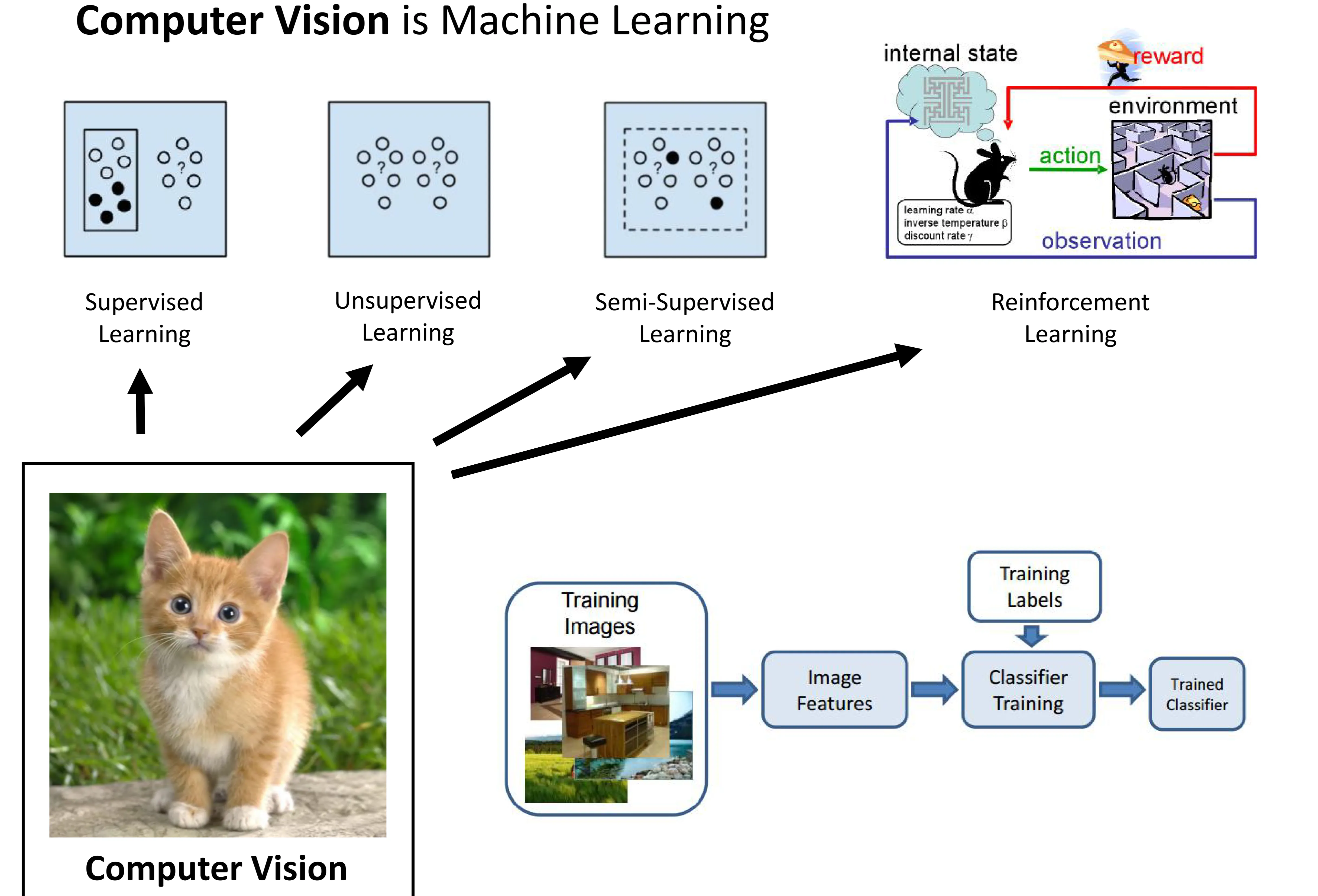
Computer Vision tasks often utilize various Machine Learning paradigms:
- Supervised Learning: Learning from labeled data. (e.g., image classification where images are labeled with object names). This is the most common approach for tasks shown in the pipeline.
  - Pipeline: Training Images → Extract Image Features → Classifier Training (using Training Labels) → Trained Classifier.
- Unsupervised Learning: Learning patterns from unlabeled data. (e.g., clustering similar images together without predefined categories).
- Semi-Supervised Learning: Learning from a mix of labeled and unlabeled data.
- Reinforcement Learning: Learning through trial and error via rewards and penalties based on actions taken in an environment. (e.g., training an agent to navigate based on visual input).

1.4 Core ML Tasks in CV

Regression: The output variable takes continuous values. (e.g., predicting the angle of steering wheel from an image).
Classification: The output variable takes discrete class labels. (e.g., identifying the object in an image as “cat”, “dog”, or “hat”).
- Note: Underneath, classification models often produce continuous values (like probabilities) representing the likelihood of belonging to each class.

2. The Challenge of Computer Vision

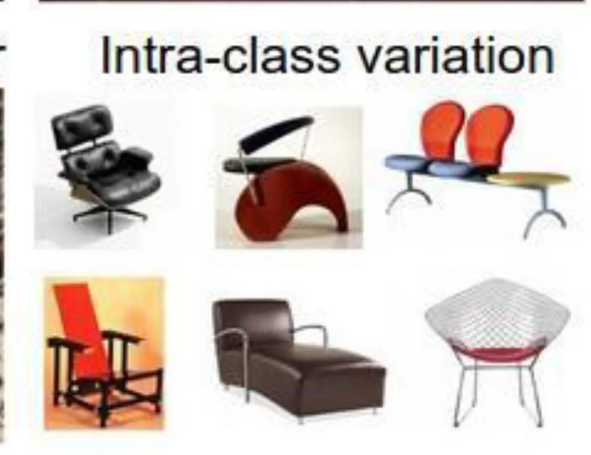
2.3 Why Computer Vision is Hard: Sources of Variation

(Diagram Description: Multiple grids of images illustrating various challenges.)

CV is difficult for computers due to numerous variations present in real-world images:
- Viewpoint variation: Objects look different from different angles.
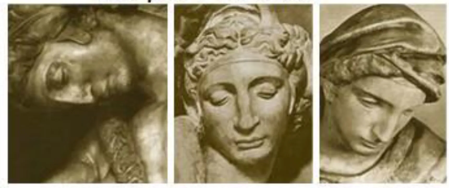
- Scale variation: Objects appear at different sizes.
- Deformation: Objects can be non-rigid and change shape.
- Occlusion: Objects can be partially hidden.
- Illumination conditions: Lighting affects object appearance drastically.
- Background clutter: Objects can blend into a complex background.
- Intra-class variation: Objects within the same category can look very different.

3. Image Classification: Pipeline and Datasets

3.1 Image Classification Pipeline (Revisited)

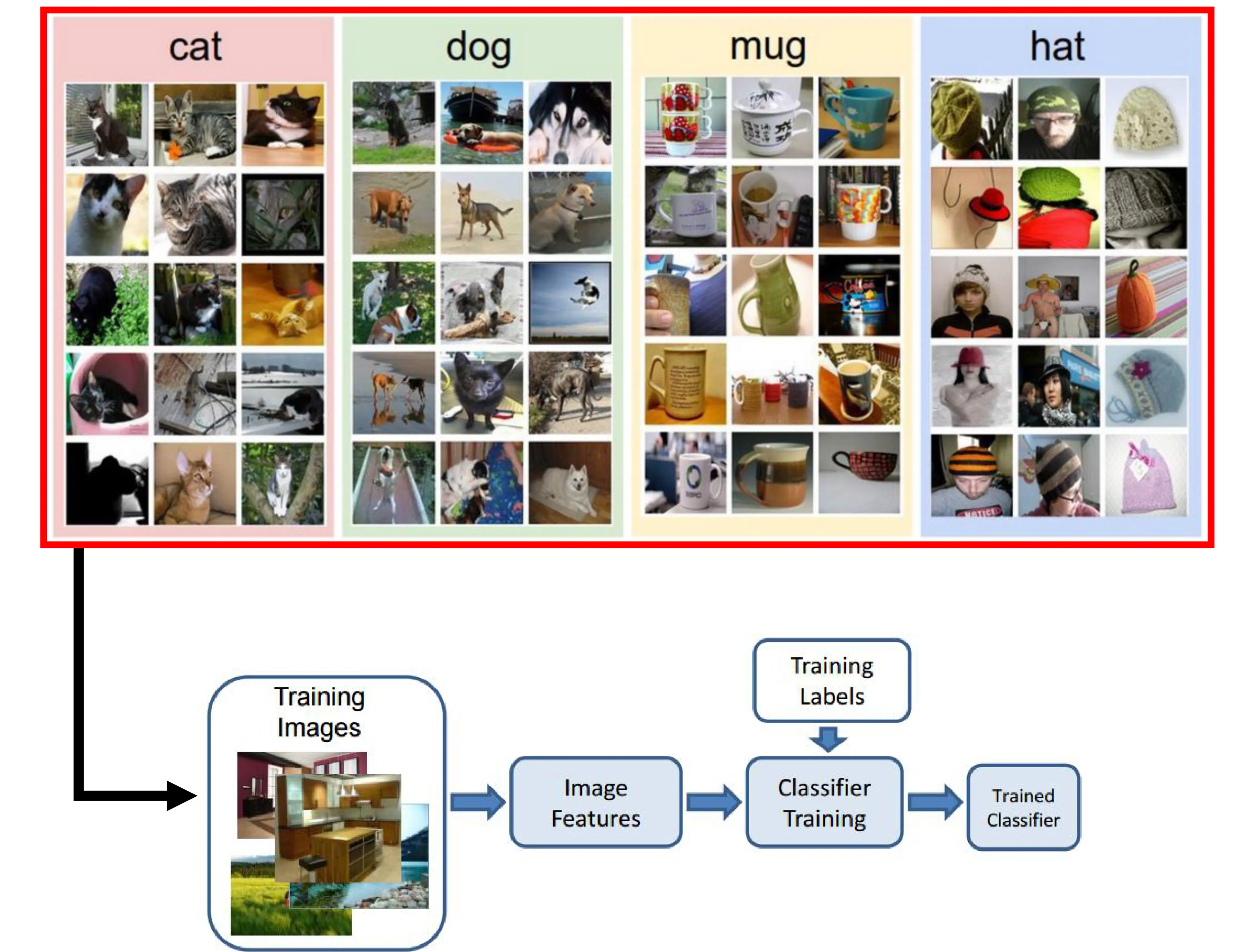
Goal: Assign a label (e.g., “cat”, “dog”) to an input image.
Standard Pipeline:
1. Input: Training Images (labeled examples).
2. Feature Extraction: Extract meaningful features (historically hand-crafted, now learned by Deep Learning).
3. Classifier Training: Train a model using features and labels.
4. Output: Trained Classifier capable of predicting labels for new images.

3.2 Famous Computer Vision Datasets

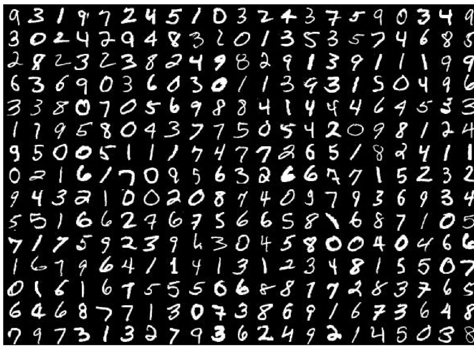
MNIST: Handwritten digits ( $0 - 9$ ). Grayscale images. Often used as a basic benchmark.
ImageNet: Large-scale dataset based on WordNet hierarchy. Over $14$ million images, $21, 841$ categories. Used in the ILSVRC challenge.
- Dataset Details: Contains links to images, not the images themselves.
- Example Hierarchy: High-level category “fruit” has $188, 000$ images. Sub-category “Granny Smith apples” has $1206$ images.
CIFAR-10 / CIFAR-100: Datasets of small ( $32 \times 32$ ) color images. CIFAR-10 has 10 classes, CIFAR-100 has 100 classes.
Places: Large-scale dataset focused on scene recognition (e.g., “kitchen”, “beach”, “street”).

4. Simple Classifier: Image Difference & K-Nearest Neighbors

4.1 Building a Classifier for CIFAR-10

Task: Classify $32 \times 32$ color images into 10 categories. (Image: CIFAR-10 examples)

4.2 Image Difference Classifier (Nearest Neighbor with L1/L2)

Concept: Compare a test image to every training image and find the closest match based on pixel differences. Assign the label of the closest training image.
Pixel-wise Distance:
- L1 Distance (Manhattan Distance): Sum of absolute differences between corresponding pixels.
  - $d_{1} (I_{1}, I_{2}) = \sum_{p} ∣ I_{1}^{p} - I_{2}^{p} ∣$ (where $p$ indexes pixels)
  - (Example Calculation:
    - Test Image Patch (Top-Left $2 \times 2$ ): $(56903223)$
    - Training Image Patch (Top-Left $2 \times 2$ ): $(1082010)$
    - Pixel-wise Absolute Differences: $(∣56 - 10∣ ∣90 - 8∣ ∣32 - 20∣ ∣23 - 10∣) = (46821213)$
      - Summing all differences across the entire image gives the L1 distance. The example shows a simplified sum of $456$ for $4 \times 4$ patches shown.*
      $test image = 569024232232601012817825518133200220$ $training image = 10812420101632248917823317100170112$ $pixel-wise absolute differences = 468212212131032143902213330108$ $L1 distance = Sum of elements = 46 + 12 + 14 + 1 + 82 + 13 + 39 + 33 + 12 + 10 + 0 + 30 + 2 + 32 + 22 + 108 = 456$
- L2 Distance (Euclidean Distance): Square root of the sum of squared differences between corresponding pixels.
  - $d_{2} (I_{1}, I_{2}) = \sum_{p} (I_{1}^{p} - I_{2}^{p})^{2}$
CIFAR-10 Accuracy:
- Random Guessing: $10%$
- Image-Diff (L1): $38.6%$
- Image-Diff (L2): $35.4%$

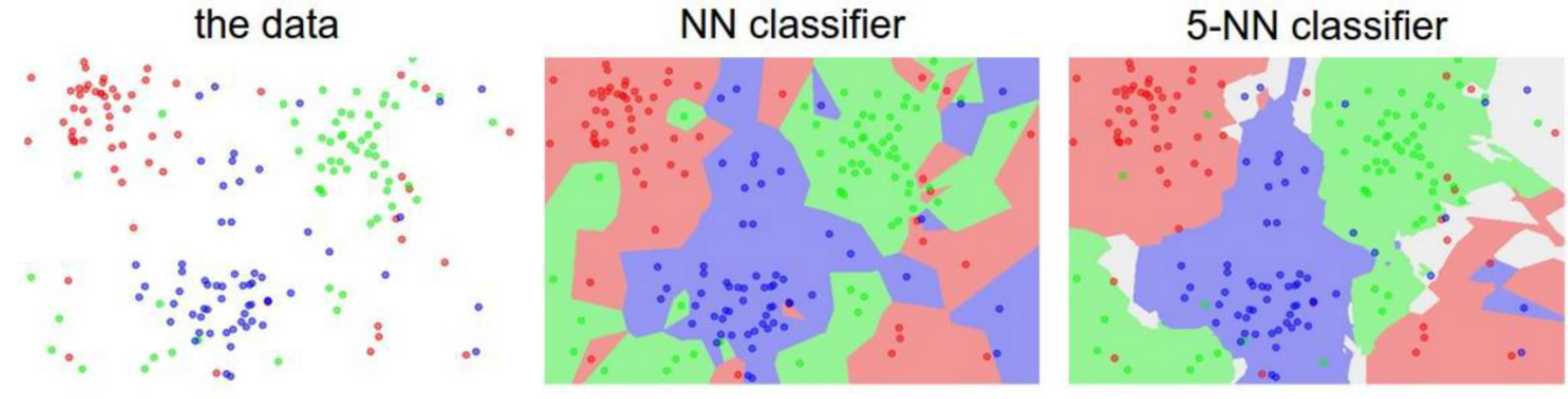
4.3 K-Nearest Neighbors (KNN)

Concept: Generalization of the simple image difference classifier. Instead of just finding the single nearest neighbor, find the $K$ nearest neighbors and have them vote for the class label.
Hyperparameters: Values set before training, like $K$ in KNN or the distance metric (L1/L2).
Tuning Hyperparameters: Finding the best hyperparameter values.
- Problem: Cannot use the test set for tuning (prevents evaluating true generalization).
- Solution: Cross-Validation:
  1. Split training data into folds (e.g., 5 folds).
  2. Train on $4$ folds, validate on $1$ fold. Repeat $5$ times, holding out a different fold each time.
  3. Average the validation performance across folds for a given hyperparameter value.
  4. Choose the hyperparameter value that performed best on average during cross-validation.
  5. Finally, train the model on the entire training set using the best hyperparameter. Evaluate on the test set once.
  - (Diagram: Training data split into ‘fold 1’…‘fold 5’ and ‘test data’)
- (Diagram: Plot of Cross-validation accuracy vs. k for KNN on CIFAR-10. Shows peak accuracy around k=7)
CIFAR-10 Accuracy with KNN:
- Training and testing on the same data (using L2): $35.4%$ (Overfits)
- 7-Nearest Neighbors (tuned via cross-validation): ~ $30%$
- Human Performance: ~ $94%$
- Convolutional Neural Networks (CNNs): ~ $95%$ (Spoiler: Much better!)

5. Neural Networks Fundamentals (Reminders)

5.1 Reminder: Weighing the Evidence (Perceptron/Neuron)

Neuron Model: Takes multiple inputs, computes a weighted sum, adds a bias, and applies an activation function.
Process:
1. Weigh: Multiply each input ( $x_{j}$ ) by its weight ( $w_{j}$ ).
2. Sum up: Calculate the weighted sum $\sum_{j} w_{j} x_{j}$ and add bias $b$ .
3. Activate: Apply a non-linear activation function $f$ (e.g., sigmoid, step function) to produce the output. $o u tp u t = f (\sum_{j} w_{j} x_{j} + b)$ .
Simple Threshold Activation: $o u tp u t = {01 if \sum_{j} w_{j} x_{j} \leq threshold if \sum_{j} w_{j} x_{j} > threshold$ (Note: Bias $b$ can be incorporated into the threshold.)

5.2 Reminder: “Learning” is Optimization of a Function

(Diagram Description: Block diagram showing forward/backward pass. Input image → differentiable block (NN) → log probabilities. Correct label influences gradients, used in backward pass to update weights. Also shows a 3D plot of a loss function surface with a minimum.)

Learning: Adjusting the model’s parameters (weights $w$ and biases $b$ ) to minimize a loss function, which measures how poorly the model performs on the training data.
Supervised Learning Process:
1. Forward Pass: Input data goes through the network to produce an output (e.g., class probabilities or scores $a$ ).
2. Loss Calculation: Compare the output $a$ to the ground truth label $y (x)$ using a loss function $C (w, b)$ .
3. Backward Pass (Backpropagation): Calculate the gradients of the loss function with respect to the parameters ( $w, b$ ). Gradients indicate the direction to adjust parameters to decrease the loss.
4. Parameter Update: Update weights and biases using an optimization algorithm (like Gradient Descent) based on the calculated gradients.
Loss Function Example (Mean Squared Error - often used in regression, related to classification losses):
- $C (w, b) = \frac{1}{2 n} \sum_{x} ∣∣ y (x) - a ∣ ∣^{2}$
- Where $n$ is the number of training examples, $y (x)$ is the ground truth label vector for input $x$ , and $a$ is the network’s output vector.
Ground Truth Example (for digit “6” in MNIST):
- $y (x) = (0, 0, 0, 0, 0, 0, 1, 0, 0, 0)^{T}$ (One-hot encoded vector)

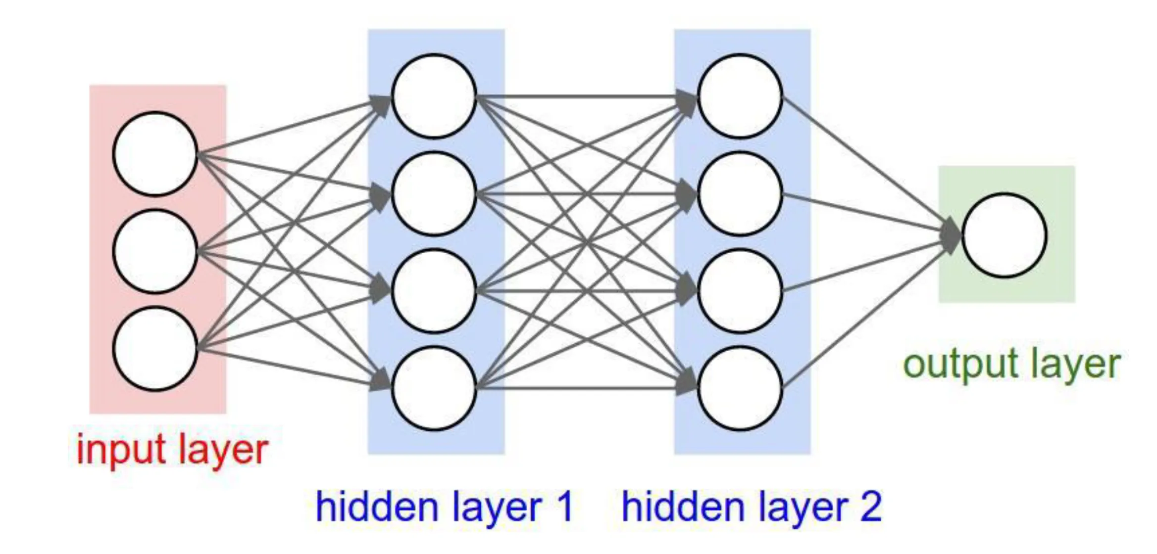
5.3 Example: Neural Network for MNIST

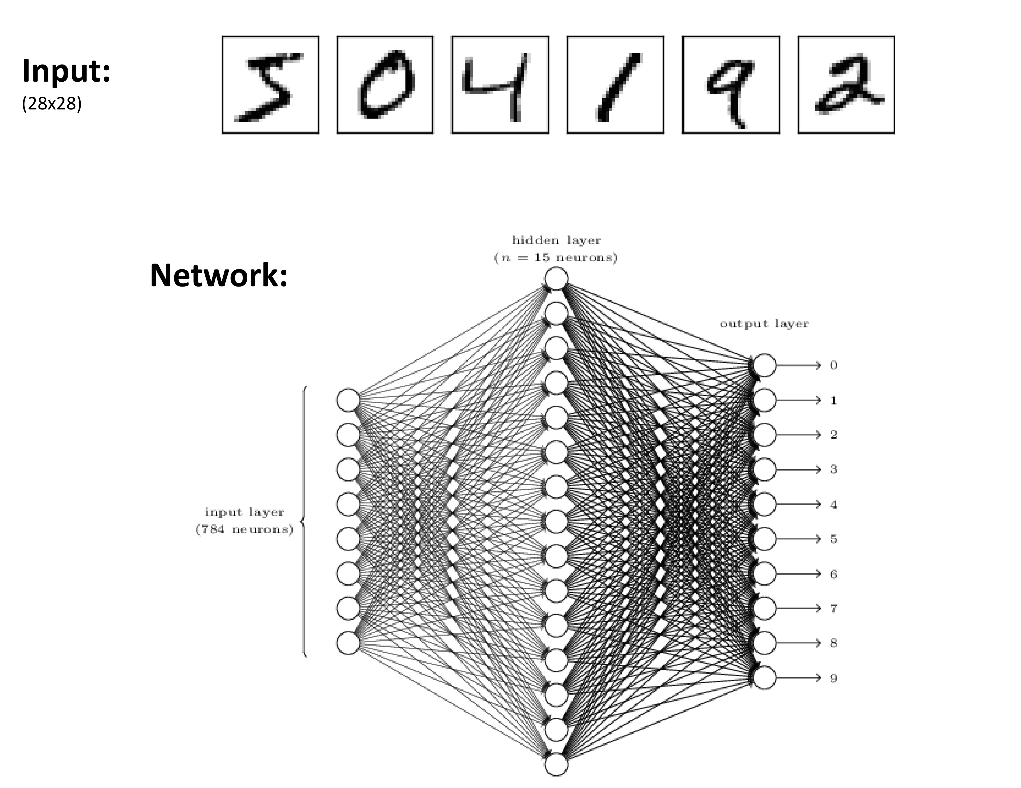
Input: Flattened MNIST image ( $28 \times 28 = 784$ pixels).
Network:
- Input Layer: $784$ neurons.
- Hidden Layer: Fully connected layer with $n = 15$ neurons (example).
- Output Layer: Fully connected layer with $10$ neurons, each corresponding to a digit class ( $0$ through $9$ ). Outputs often represent class scores or probabilities (after softmax).

6. Convolutional Neural Networks (CNNs)

6.1 Introduction to CNNs

Regular Neural Network (Fully Connected): Neurons in one layer are connected to all neurons in the next layer. Treats input (like an image) as a flat vector. Does not account for spatial structure.
Convolutional Neural Network: Designed specifically for processing grid-like data, such as images. Takes advantage of spatial structure.
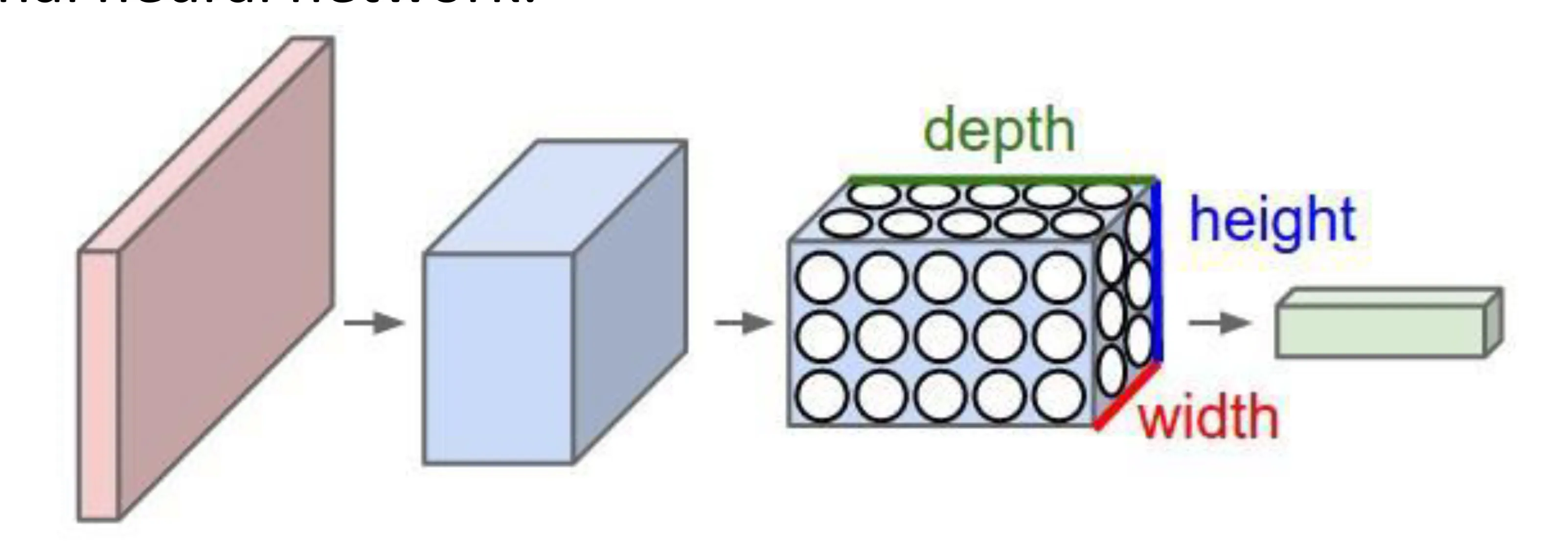
- Layers process data in 3D volumes: depth, height, width.
- Each layer transforms an input 3D volume to an output 3D volume using a differentiable function (which may or may not have learnable parameters).

6.2 CNN Layers

Common Layers:
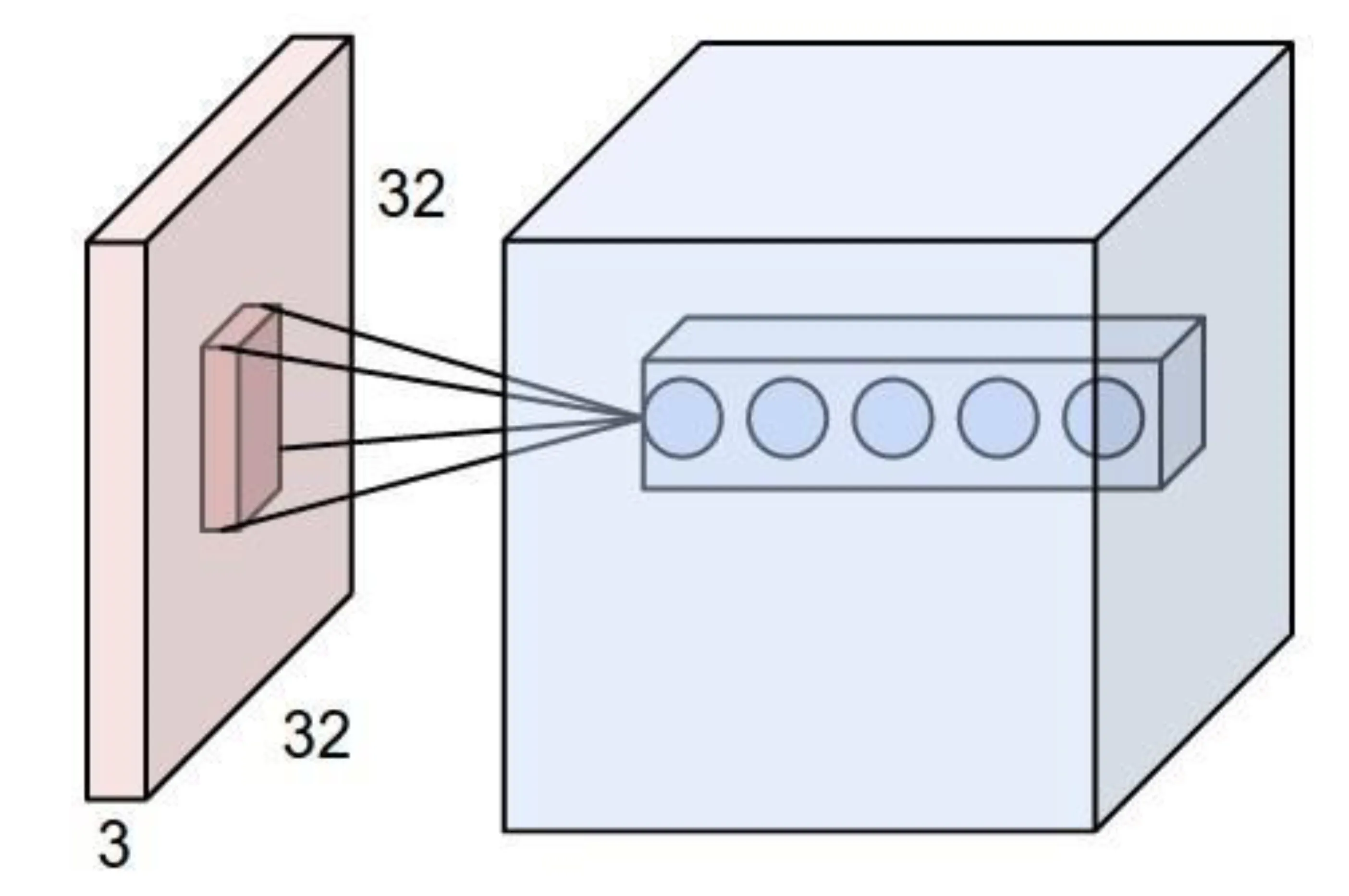
- INPUT e.g., $32 \times 32 \times 3$ : Holds raw pixel values of the input image. Dimensions are (height $\times$ width $\times$ depth/channels). Depth is $3$ for R, G, B color channels.
- CONV (Convolutional Layer): Computes output of neurons connected to local regions in the input volume (receptive field). Performs convolutions (dot products between filter weights and input regions). Preserves spatial structure.
  - Learnable parameters: Filters (weights) and biases.
  - Example output volume: $[32 \times 32 \times 12]$ if using $12$ filters.
- RELU (Rectified Linear Unit): Element-wise activation function. Applies $ma x (0, x)$ . Introduces non-linearity without changing volume size.
  - No learnable parameters.
  - Example output volume: $[32 \times 32 \times 12]$ (same as input).
- POOL (Pooling Layer): Downsamples the volume along spatial dimensions (width, height). Reduces computation, increases robustness to small spatial variations. Common types: Max Pooling, Average Pooling.
  - No learnable parameters.
  - Example output volume: $[16 \times 16 \times 12]$ (downsampled width/height).
- FC (Fully-Connected Layer): Standard neural network layer where each neuron is connected to all numbers in the previous volume. Usually found near the end of the network for classification.
  - Learnable parameters: Weights and biases.
  - Example output volume: $[1 \times 1 \times 10]$ for 10 class scores (e.g., in CIFAR-10). Each of the $10$ numbers corresponds to a class score.

6.3 CONV Layer: Local Connectivity

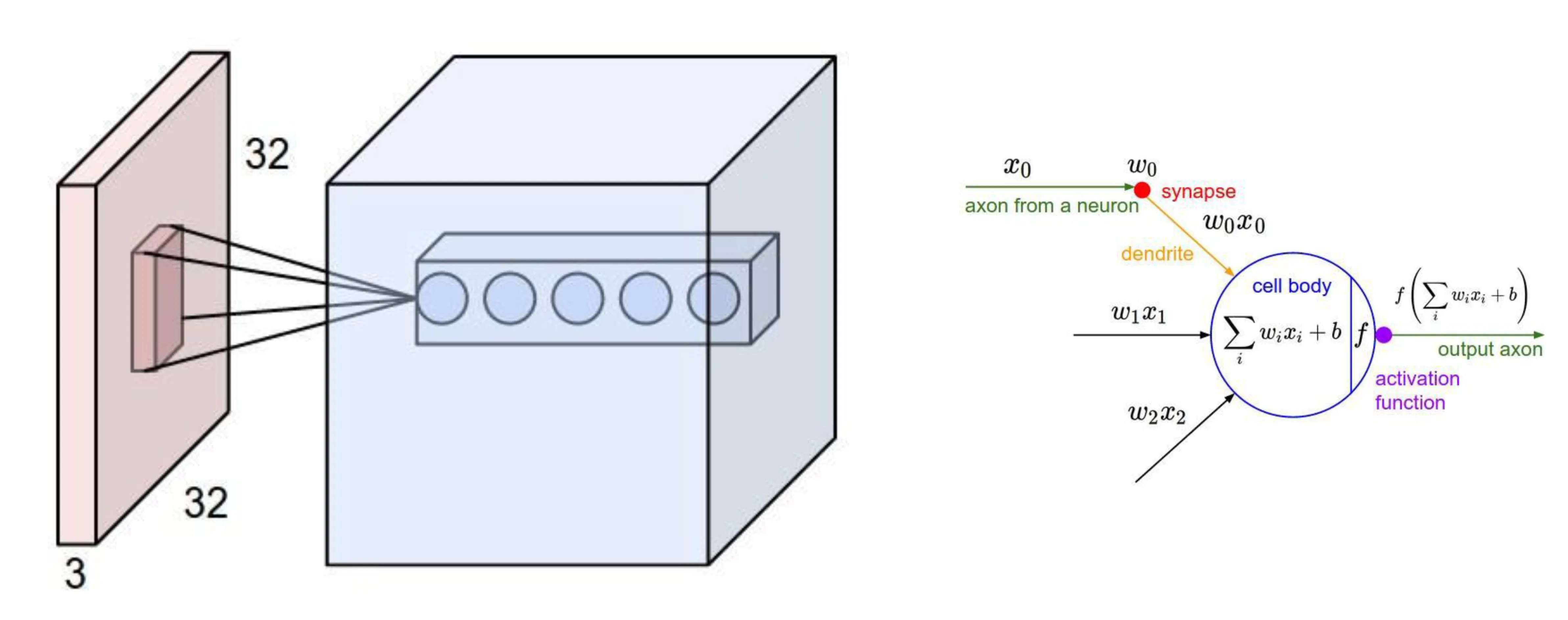
Neurons in a CONV layer are only connected to a small, local region of the input volume (their receptive field).
The extent of this connectivity is determined by the filter size.
This contrasts with FC layers where neurons connect to the entire input.

The same set of weights (the filter or kernel) is used for all neurons within the same depth slice of the output volume.
Neurons at different spatial locations ( $x, y$ ) in the same output slice use the identical filter, just applied to different input patches.
Rationale: If a feature detector (like a horizontal edge detector) is useful in one part of the image, it’s likely useful in other parts too.
Dramatically reduces the number of parameters compared to FC layers.

6.5 CONV Layer: Spatial Arrangement of Output Volume

The output volume’s dimensions are controlled by three hyperparameters:
- Depth: Number of filters used. Each filter learns to detect a different feature. The output volume will have a depth equal to the number of filters.
- Stride ( $S$ ): Step size the filter takes as it slides across the input volume. Larger stride produces smaller output spatial dimensions.
- Padding ( $P$ ): Amount of zero-padding added around the border of the input volume. Often used to control the output spatial dimensions (e.g., preserve input width/height).
Output Size Calculation (Width or Height):
- Given input size $W$ , filter size $F$ , stride $S$ , padding $P$ .
- Output size $W_{o u t} = \frac{( W - F + 2 P )}{S} + 1$
- (Must result in an integer).

6.7 Example Convolution Filters

Identity: Outputs the original image (approximately). $000010000$
Edge Detection: Detects edges/gradients. $10 - 1 000 - 1 01 or 010 1 - 4 1 010 or - 1 - 1 - 1 - 1 8 - 1 - 1 - 1 - 1$

6.8 Convolution as Representation Learning

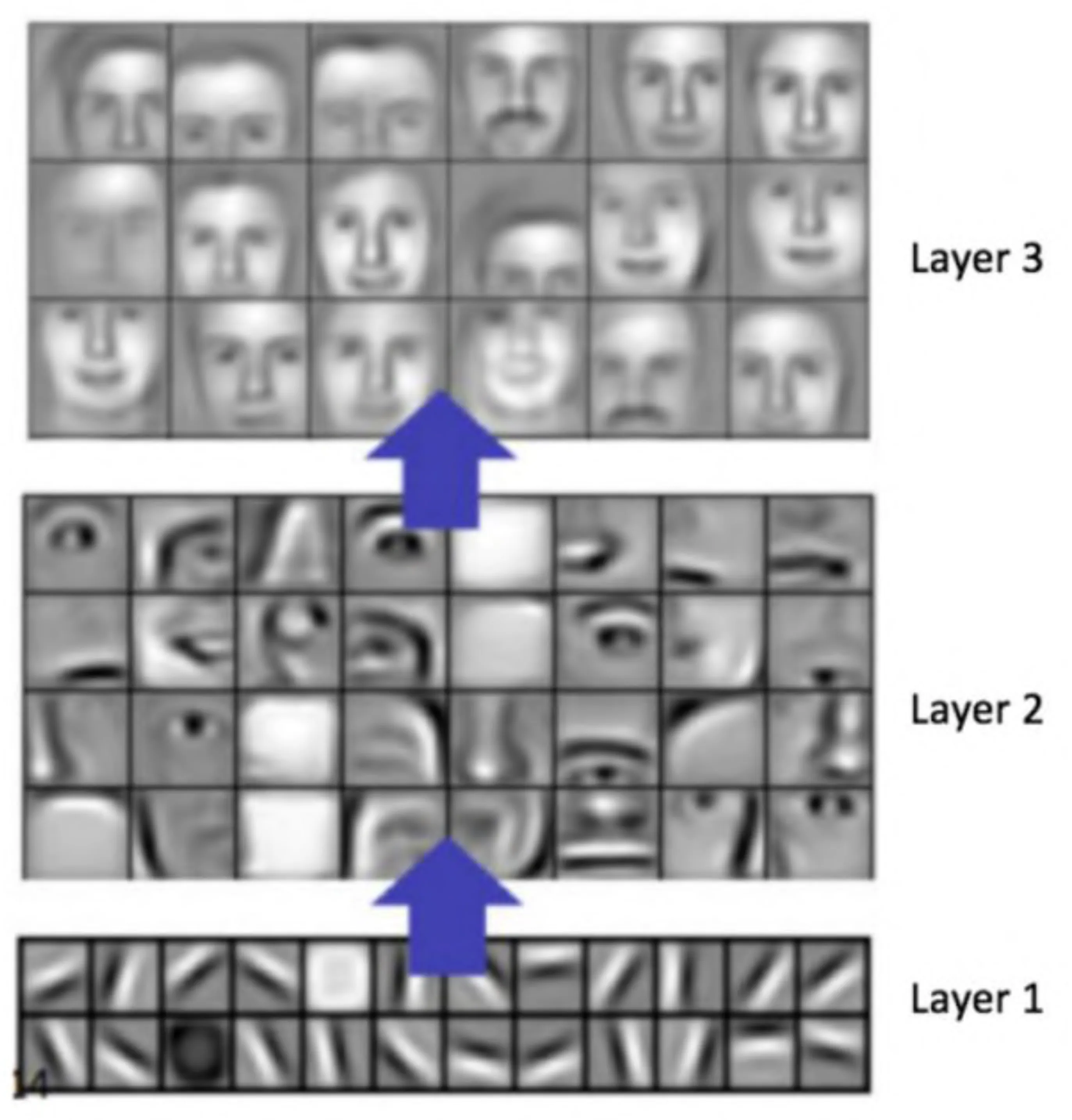
CNNs learn hierarchical representations automatically.
Layer 1: Learns basic features like edges, corners, color blobs. (Image: Grid of Gabor-like filters)
Layer 2: Combines Layer 1 features to learn more complex patterns like textures, parts of objects (e.g., eyes, noses).
Layer 3 (and deeper): Combines Layer 2 features to learn representations of object classes.

6.9 POOL Layer: Pooling

Purpose: Reduce spatial dimensions (width, height) of the volume. Makes representation more robust to small translations and distortions. Reduces computational cost.
Max Pooling: Slides a window over the input volume slice and takes the maximum value within that window.
Example: Max pool with $2 \times 2$ filters and stride $2$ .
- Input Slice: $1531162227134804$
- Output Slice: $[max (1, 1, 5, 6) max (3, 2, 1, 2) max (2, 4, 7, 8) max (1, 0, 3, 4)] = [6384]$
Reduces width and height, keeps depth the same.
Example Volume Downsampling: $224 \times 224 \times 64 pool 112 \times 112 \times 64$ .

7. CNN Architectures and Applications

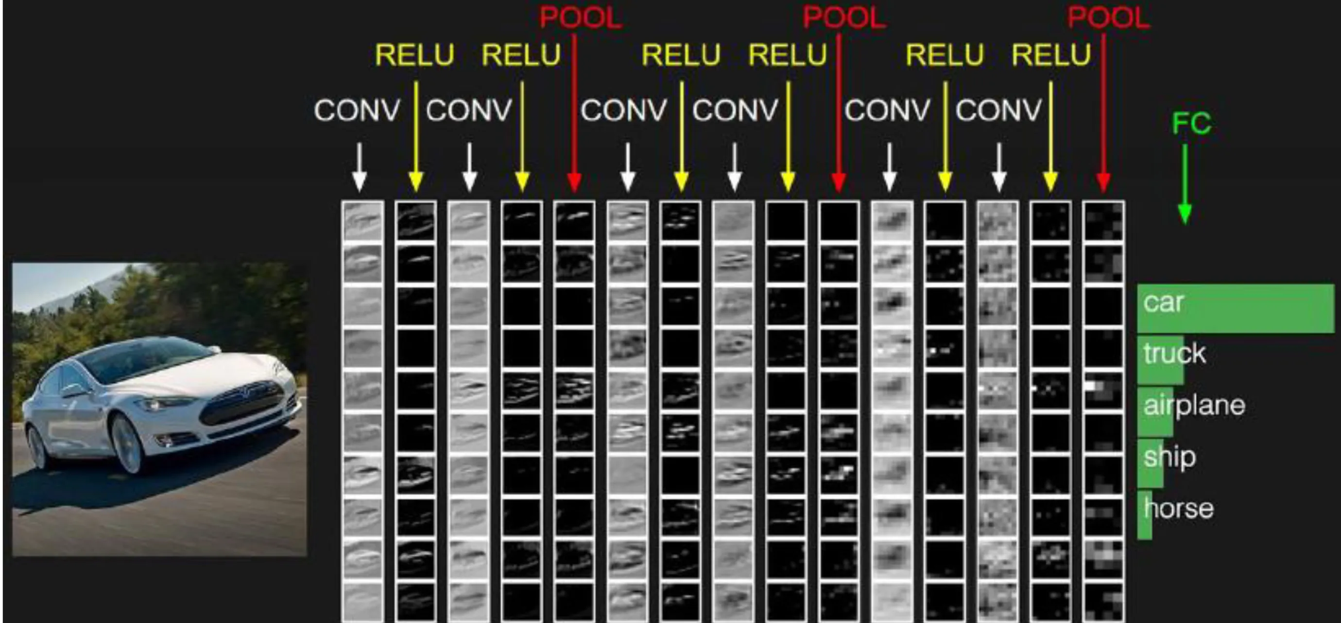
7.1 Generic CNN Architecture for Classification

(Diagram: Input → [CONV → RELU → POOL] repeating → FC → Output)*

A common pattern involves stacking CONV, RELU, and POOL layers, followed by one or more FC layers for final classification.

7.2 Adaptable Architecture for Many Applications

The core CNN architecture (convolutional base) acts as a powerful feature extractor.
The final layers can be modified for different tasks beyond simple classification:
- Different Image Classification Domains: Use the same architecture, retrain/fine-tune on new domain data.
- Image Captioning: Add Recurrent Neural Networks (RNNs) like LSTMs to generate sequences (text descriptions).
- Image Object Localization: Output bounding box coordinates ( $x, y, w, h$ ) in addition to class labels.
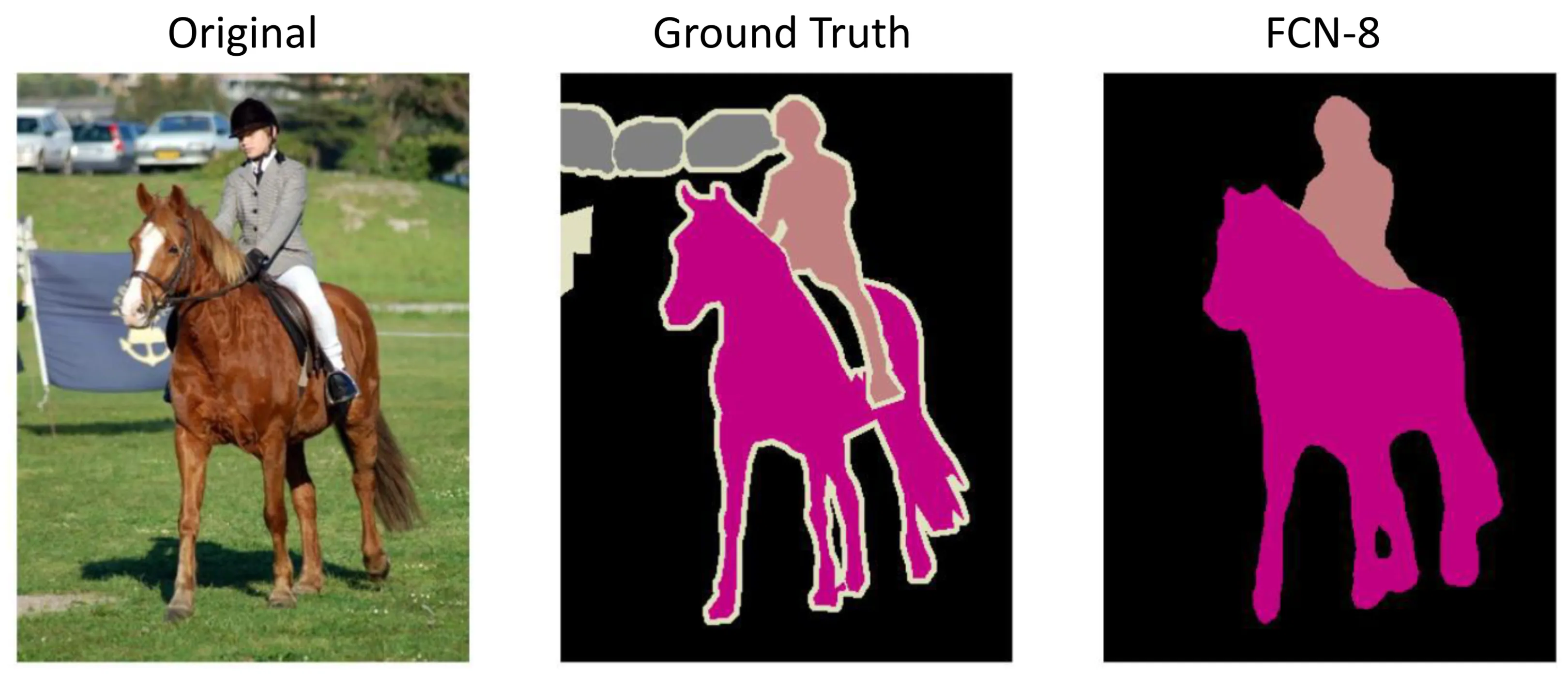
- Image Segmentation: Use Fully Convolutional Networks (FCNs) or Deconvolution Layers to output a prediction for every pixel (semantic segmentation).

7.3 Case Study: ImageNet (ILSVRC)

ImageNet Large Scale Visual Recognition Challenge (ILSVRC): Annual competition driving progress in CV, particularly object classification and detection.
Dataset: Subset of ImageNet, typically $1.2$ million training images, $50, 000$ validation images, $100, 000$ test images, for $1000$ object categories.
Evaluation Metric (Classification): Top-5 Error Rate
- The model predicts probabilities for all $1000$ classes.
- It gets credit if the correct label is among its top $5$ predictions.
- Top-5 error is the percentage of test images where the correct label is not in the top 5.
- (Diagram: Example showing ground truth “Steel drum”, one prediction getting Accuracy: 1 (correct label in top 5), another getting Accuracy: 0)
- Top-5 error is significantly lower than Top-1 error (e.g., ~20% reduction mentioned for AlexNet 2012).
Human Performance: Humans annotated the test set using a binary task (“apple” or “not apple”), achieving very low error rates (often cited around $5%$ , later models surpassed this).

7.4 Evolution of CNN Architectures on ImageNet

(Diagram: Bar chart showing decreasing Top-5 error rate from 2012 to 2015/2016)

AlexNet (2012): First major CNN success on ILSVRC.
- Top-5 Error: $15.4%$ (originally 16.4% shown in chart)
- Architecture: $8$ layers (5 CONV, 3 FC). Used RELU, Dropout, Data Augmentation.
- Parameters: $61$ million.
- (Diagram: AlexNet layer structure C1, P1, N1… FC8)
ZFNet (2013): Improvement on AlexNet by tuning hyperparameters, especially filter size and stride in early layers. Visualized features.
- Top-5 Error: $11.2%$ (originally 11.7% shown)
- Architecture: $8$ layers. More filters, denser stride.
VGGNet (2014): Showed depth is critical. Very uniform architecture.
- Top-5 Error: $7.3%$
- Architecture: $16$ or $19$ layers. Used only small $3 \times 3$ CONV filters (stacked) and $2 \times 2$ POOL layers.
- Parameters: $138$ million (very large).
- (Diagram: VGGNet vs AlexNet structure, VGG’s uniform blocks)
GoogLeNet (2014): Focused on computational efficiency while increasing depth. Introduced Inception Module.
- Top-5 Error: $6.7%$
- Architecture: $22$ layers. Used Inception modules which perform convolutions with multiple filter sizes ( $1 \times 1, 3 \times 3, 5 \times 5$ ) in parallel and concatenate results. Used global average pooling instead of final FC layers.
- Parameters: $5$ million (much smaller than AlexNet/VGG).
- (Diagram: Overall GoogLeNet structure with stacked Inception modules. Detail of one Inception module.)
ResNet (Residual Network) (2015): Enabled training of much deeper networks using Residual Connections (Skip Connections). Addressed vanishing gradient problem in very deep networks.
- Top-5 Error: $3.57%$ (First to surpass reported human-level performance on this specific task)
- Architecture: Up to $152$ layers. Residual blocks learn $F (x) = H (x) - x$ , where input $x$ is added back via a skip connection: $H (x) = F (x) + x$ . Easier to learn identity mapping.
- Parameters: Varies with depth. More layers generally led to better performance.
- (Diagram: Plain vs Residual network comparison. Detail of a residual block with skip connection.)
CUImage (2016): Further improvements, often using ensembles (combining multiple models).
- Top-5 Error: $2.99%$
- Method: Ensemble of $6$ models (likely ResNet variants or similar).

7.5 Other Advanced Applications

Segmentation:
- Semantic Segmentation: Classify every pixel in an image.
- Fully Convolutional Networks (FCNs): Replace FC layers in classification networks with CONV layers to produce heatmaps. Upsample heatmap to get pixel-wise predictions.
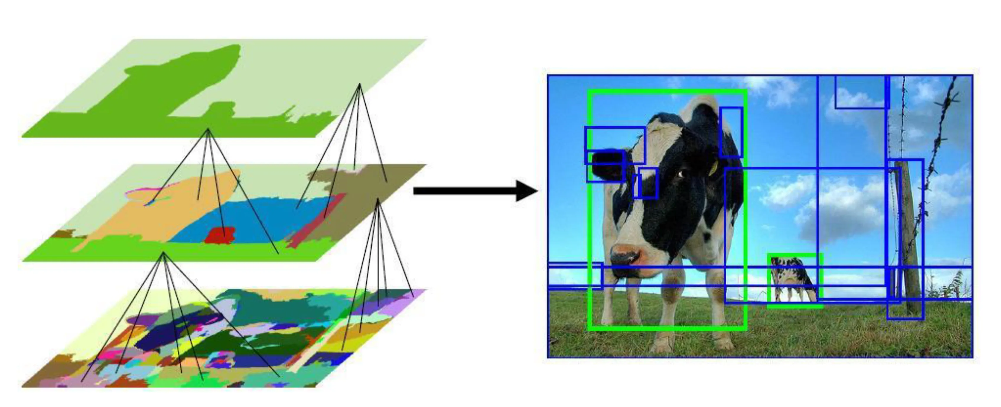
Object Detection: Identify object classes and locate them with bounding boxes.
- R-CNN (Regions with CNN features):
  1. Propose candidate regions (~ $2 k$ ) using selective search.
  2. Warp each region to fixed size.
  3. Extract CNN features (e.g., from AlexNet) for each warped region.
  4. Classify regions using SVMs.
  5. Refine bounding boxes using regression.
Image Caption Generation: Generate a natural language description of an image.
- Often uses a CNN (feature extractor) combined with an RNN/LSTM (sequence generator). Attention mechanisms often used.
- (Diagram: Example image “man sitting on a couch with a dog” with generated captions. Attention visualization highlighting image regions corresponding to words “dog”, “man”, “sitting”, “couch”. Pipeline: detect words → generate sentences → re-rank sentences)
Image Question Answering (VQA): Answer natural language questions about an image.
- Combines CNN (for image features) and RNN/LSTM (for question encoding) to predict an answer.
- (Diagram: Example questions/answers for different images. VQA model architecture: Image→CNN, Question→WordEmbedding→LSTM, combined features → Softmax → Answer)
- Code: https://github.com/renmengye/imageqa-public
Video Description Generation: Generate captions for video clips.
- Uses CNNs for frame-level features combined with RNNs/LSTMs across time to generate descriptions.
- (Diagram: S2VT (Sequence-to-Sequence Video to Text) architecture. Examples of correct/incorrect descriptions for videos.)
- Code: https://vsubhashini.github.io/s2vt.html
Modeling Attention Steering: Models that learn where to look in an image sequentially to perform a task (like object recognition).
- Recurrent Attention Model (RAM): Uses RNNs to decide the next “glimpse” location based on past glimpses.
- (Diagram: Examples of attention glimpses on digits. RAM architecture diagram.)
Audio Classification: Applying CNNs (often 1D CNNs or 2D CNNs on spectrograms) to audio tasks.
- (Diagram: Spectrograms comparing “Dry Road” vs. “Wet Road” tire noise)
Driving Scene Segmentation: Semantic segmentation applied to autonomous driving context.
- (Diagram: Driving scene image and its pixel-wise segmentation into classes like Sky, Building, Road, Pavement, Tree, Car, Pedestrian, etc.)
End-to-End Learning of Driving Task: Training a model (often CNN) to directly predict driving controls (e.g., steering angle) from raw sensor input (e.g., camera images).
- (Diagram: Comparison of human/Tesla control vs. learned control steering wheel visualizations. Plot of steering angle over time.)
- Project: http://cars.mit.edu/deeptesla

7.6 Vision for Intelligent Systems Hierarchy

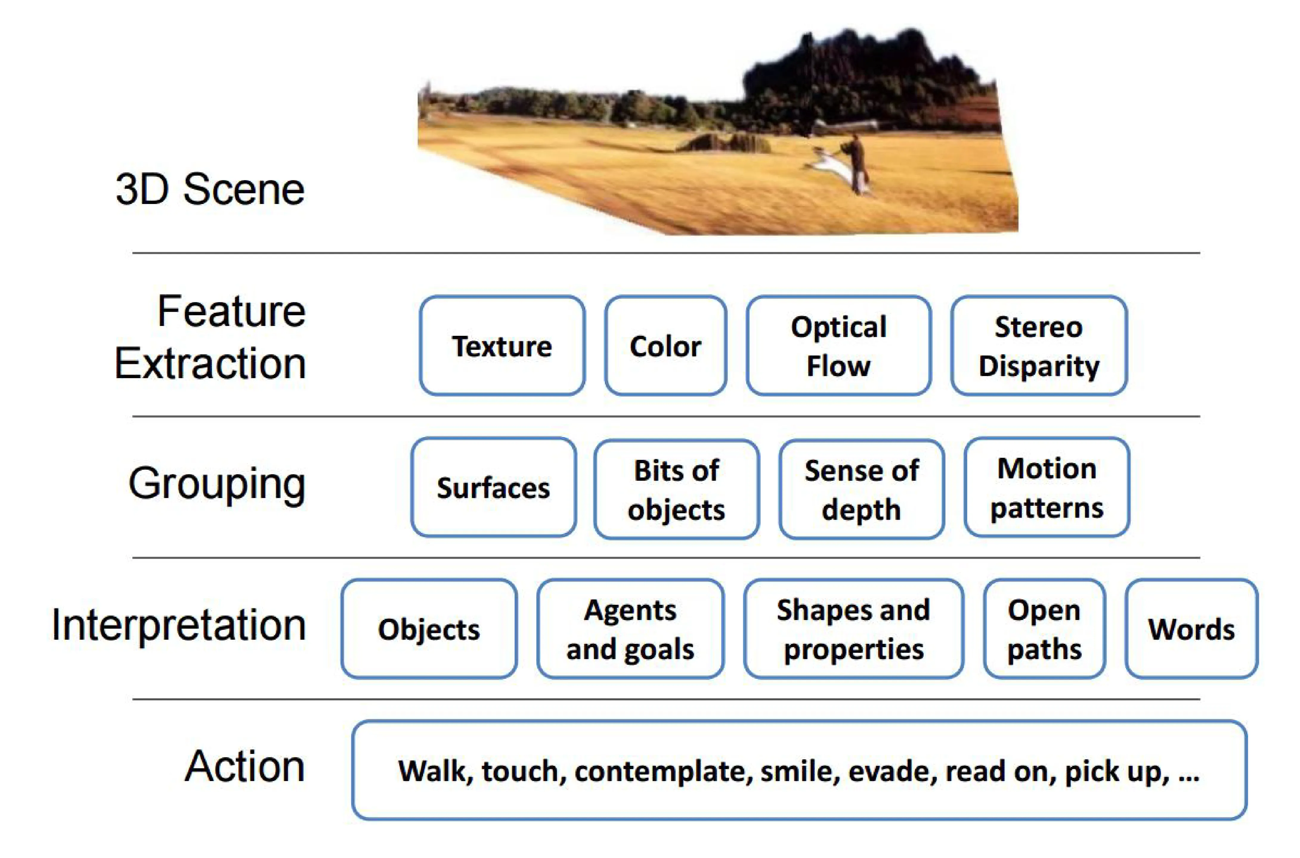
3D Scene: The physical world.
Feature Extraction: Detect low-level features (Texture, Color, Optical Flow, Stereo Disparity).
Grouping: Group features into surfaces, bits of objects, infer depth, motion patterns.
Interpretation: Recognize objects, agents/goals, shapes/properties, open paths, understand semantics (Words).
Action: Interact with the world (Walk, touch, contemplate, smile, evade, read on, pick up, …).

8. Open Problems and Challenges

8.1 Robustness: Adversarial Examples

Deep neural networks can be surprisingly fragile and non-robust.
Problem 1: High Confidence on Unrecognizable Images:
- Networks can be fooled into classifying meaningless noise patterns or generated patterns as real objects with extremely high confidence ( $> 99.6%$ ).
- (Image: Noise patterns confidently classified as “robin”, “cheetah”, “armadillo”, “lesser panda”. Geometric/texture patterns classified as “king penguin”, “starfish”, “baseball”, “electric guitar”.)
- Reference: Nguyen et al. 2015
Problem 2: Fooled by Small Distortions:
- Adding carefully crafted, often imperceptible, perturbations to a legitimate image can cause the network to misclassify it completely.
- (Image: Original image (e.g., school bus) classified correctly. Adding small distortion causes it to be misclassified as “ostrich”.)
- Reference: Szegedy et al. 2013

8.2 Object Category Recognition Challenges (Examples)

(Images: Series of cat photos illustrating challenges)

Occlusion (Cat behind table leg, cat peeking from behind tree).
Unusual poses/context (Cat paw reaching into food bowl).
Challenging appearance (Cat wearing a lion mane, cat in a monkey suit). These highlight the need for robustness against variations not well-represented in standard training sets.

Quartz 4

Explorer

Deep Learning for Computer Vision (MIT Course 6.S191 - Jan 2017)