Edge Detection & Boundary Tracing

Edge Detection

Edge detection aims to identify points in a digital image at which the image brightness changes sharply or has discontinuities. These points typically correspond to boundaries between objects or regions.

Edge Detection Methods Overview

1. **Discrete Approximation of Gradient & Thresholding:**k

   • Calculate the gradient (first derivative) of the image intensity.
   • Compute the gradient magnitude (norm).
   • Apply a threshold to the gradient magnitude image.
   • Edge Definition: Points with a large gradient magnitude are considered edges.

2. Second Derivative & Zero Crossing Detection:

   • Utilizes the second derivative (e.g., Laplacian).
   • Edge Definition: Edges correspond to zero-crossings in the second derivative image, specifically at locations where the first derivative (gradient) has a maximum or minimum along the gradient direction.
   • Advantages: Detects weak edges (gradual variations) better than simple gradient thresholding. Less chance of multiple edge responses for a single boundary.
   • Disadvantage: More sensitive to noise.

3. Derivative Issues:

   • Differentiation enhances noise present in the image.
   • The second derivative enhances noise even more than the first derivative.

4. Band-Pass Filtering (Smoothing + Derivative):

   • Combines smoothing (to reduce noise) with differentiation.
   • Typically involves applying a smoothing filter (like Gaussian) followed by taking the first or second derivative.
   • Example: Laplacian of Gaussian (LoG).

5. Compass Operators:

   • Use a set of masks sensitive to edges in specific orientations.

Edges in 1D

(Based on figure from http://www.pages.drexel.edu/~weg22/edge.html)

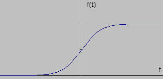
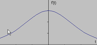
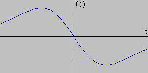
• Figure Description:
  • The first graph shows a 1D signal $f(t)$ representing an idealized, sharp step edge (transition from low to high intensity).
  • The second graph shows the first derivative $f^{\prime }(t)$ of the signal from the second graph.
  • The third graph shows the second derivative $f^{\prime \prime }(t)$ of the signal from the second graph.
• Concept Illustrated: The locations of edges (sharp changes in intensity) in the original signal $f(t)$ correspond to peaks (maxima or minima) in the magnitude of its first derivative $f^{\prime }(t)$. The zero-crossing of the second derivative (not shown, but related to the peaks/troughs of the first derivative) also indicates edge locations.

Edge Detection Operators

First Derivative Operators

• Examples: Sobel, Roberts, Prewitts operators.
• General Approach:
  • Often approximate gradient by smoothing in one direction (e.g., row-wise) and differentiating in the orthogonal direction (e.g., column-wise), and vice-versa.
  • Apply masks to compute gradient components in $x$ and $y$ directions ($G_x$, $G_y$).
  • Compute the gradient magnitude (norm), e.g., $\sqrt{G_x^2+G_y^2}$ or $|G_x|+|G_y|$.
  • Compute the gradient direction: $\theta =\text{Arctan}(\frac{G_y}{G_x})$. This direction is perpendicular to the direction of the edge itself.

Second Derivative + Smoothing Operators

• Example: Marr-Hildreth operator or Laplacian of Gaussian (LoG).
• Approach:
  1. Gaussian Prefiltering: Smooth the image with a Gaussian filter to reduce noise and select scale.
  2. Laplacian Computation: Compute the Laplacian (${\nabla }^2$) of the smoothed image. The Laplacian is a second-derivative operator, often approximated by a discrete kernel. - Laplacian in 2D: ${\nabla }^{2}f=\frac{{\partial }^{2}f}{\partial x^2}+\frac{{\partial }^{2}f}{\partial y^2}$
• Properties:
  • Works better when grayscale transitions are smooth.
  • Edges are located at the zero-crossings of the LoG output.
• Approximation: The LoG can be approximated by the Difference of Gaussians (DoG) or “Mexican hat” operator, which involves subtracting two Gaussian functions with different variances ($\sigma$).

Compass Operators

• Approach: Use a set of directional first derivative masks (often based on Sobel or Prewitts kernels rotated to different orientations, e.g., $0^{\circ },45^{\circ },90^{\circ },135^{\circ }$).
• Compute the directional derivative response for each mask.
• The maximum response across all directions gives the edge magnitude, and the mask giving the maximum response indicates the edge orientation.
• Can be used specifically to find edges of a particular orientation.

Canny’s Edge Detector

• Considered the most commonly used and often state-of-the-art edge detector (developed in 1983).
• See dedicated section below.

Canny’s Edge Detector

• Developed by John Canny (1983, MIT MS student).
• Design Goals (Optimality Criteria):
  1. Good Detection: Low probability of missing real edges (low false negatives). Low probability of falsely detecting non-edges (low false positives).
  2. Good Localization: Detected edge points should be as close as possible to the center of the true edge.
  3. Single Response: Only one response to a single edge (avoid multiple detections for one edge).
• Approach: Formulated as finding an optimal filter (within the class of linear shift-invariant operators initially) that maximizes the product of signal-to-noise ratio and a localization measure. The result approximated a first derivative of a Gaussian.

Main Steps of the Canny Algorithm

1. Noise Reduction (Smoothing):

   • Smooth the input image using a Gaussian kernel: $I_{smoothed}=G_{\sigma }\ast I$.
   • The standard deviation $\sigma$ controls the level of smoothing. Larger $\sigma$ reduces more noise but can blur/shift edges. Purpose: Reduce false alarms caused by noise.

2. Gradient Calculation:

   • Compute the image gradient using a first-derivative operator (e.g., Sobel) on the smoothed image $I_{smoothed}$.
   • Calculate Gradient Magnitude: $M=\sqrt{G_x^2+G_y^2}$
   • Calculate Gradient Direction: $\theta =\text{Arctan}(\frac{G_y}{G_x})$
   • Quantify Direction: Round the gradient angle $\theta$ to the nearest multiple of $45^{\circ }$ (representing horizontal, vertical, and two diagonal directions). This is needed for non-maximal suppression.

3. Non-Maximal Suppression (NMS):

   • Purpose: Localization - thin the edges to single-pixel width.
   • For each pixel, examine its gradient magnitude $M$.
   • Compare $M$ with the gradient magnitudes of its two neighbors along the (quantified) gradient direction $\theta$.
   • Rule: If the pixel’s magnitude $M$ is not greater than both of its neighbors along the gradient direction, suppress this pixel (set its edge magnitude to 0). Otherwise, keep it.
   • Example: If the gradient direction is horizontal, compare the pixel with its left and right neighbors. If diagonal, interpolate neighbors or use diagonal neighbors.

4. Hysteresis Thresholding:

   • Purpose: Reduce misses (connect broken edges) while still removing weak noise-related edges. Uses two thresholds:

     • $T_L$: Low threshold
     • $T_H$: High threshold (where $T_L<T_H$, often $T_H\approx 2\times T_L$)

   • Procedure: a. Classify pixels after NMS based on magnitude $M$: - If $M>T_H$: Mark as a strong edge pixel. - If $T_L<M\le T_H$: Mark as a weak edge pixel. - If $M\le T_L$: Suppress (mark as not an edge). b. Keep all strong edge pixels in the final edge map. c. Keep weak edge pixels only if they are connected (adjacent via 8-connectivity) to a strong edge pixel, either directly or through a path of other connected weak edge pixels. d. Discard all weak pixels that are not connected to strong pixels.

   • Note: The slide’s description of hysteresis (“Suppress all points with magnitude < TH”, “If a point has magnitude > TL and is linking two points with magnitude > TH, then keep it”) seems non-standard or potentially contains typos. The description above follows the widely accepted Canny hysteresis method.

Applying Canny

(Based on figure showing Lena image from http://www.pages.drexel.edu/~weg22/edge.html)

• Figure Description:
  • Left: Original Lena image.
  • Middle: Result after non-maximal suppression but before hysteresis thresholding. Edges are thinned, but some real edges might be broken (contain gaps where magnitude fell below $T_H$), and some weaker noise edges might still exist. Some edges appear missing.
  • Right: Final Canny edge map after hysteresis thresholding. Weak edges connected to strong edges are preserved, forming more continuous contours. Isolated weak edges are removed.

---

Boundary Tracing & Edge Linking

After edge detection (finding individual edge pixels) or image segmentation (separating foreground/background), we often want to organize these pixels into meaningful boundaries or contours.

Boundary Tracing

• Input: A “segmented” image, typically binary, where foreground pixels have one label (e.g., 1) and background pixels have another (e.g., 0).

• Goal: To find an ordered sequence of pixels that constitutes the boundary between the foreground region(s) and the background.

• Types of Boundaries:

  • Inner Boundary: Consists of the outermost pixels belonging to the foreground region.
  • Outer Boundary: Consists of the innermost pixels belonging to the background region, adjacent to the foreground region.

• Methods & Tools:

  • Contour Following Algorithms: Step-by-step procedures to trace the boundary pixels (see Algorithm 5.6 below).
  • Level Set Methods: Can be used if the image is represented differently (e.g., foreground=1, background=-1). Zero level set finding methods can provide subpixel boundary coordinates. (MATLAB: contour function).
  • MATLAB Functions (for binary images):
    • bwtraceboundary: Traces the boundary of a single object starting from a specified point. Finds the inner boundary.
    • bwboundaries: Finds the boundaries (inner boundaries) of all objects in a binary image. Returns a cell array, where each cell contains the coordinate list for one object’s boundary.

• Segmentation Prerequisite: Boundary tracing requires a segmented image. The simplest segmentation method is intensity thresholding (to be discussed separately).

4-connected vs 8-connected Neighbors

• Connectivity: Defines which pixels are considered neighbors to a central pixel $(x,y)$.
  • 4-connected neighbors: The pixels directly above, below, left, and right: $(x,y-1)$, $(x,y+1)$, $(x-1,y)$, $(x+1,y)$.
  • 8-connected neighbors: The 4-connected neighbors PLUS the four diagonal neighbors: $(x-1,y-1)$, $(x+1,y-1)$, $(x-1,y+1)$, $(x+1,y+1)$.
• The choice of connectivity affects how boundaries are traced and how regions are defined.

Algorithm 5.6: Inner Boundary Tracing

This algorithm traces the inner boundary (outermost pixels of the foreground region).

(Based on text description and Figure 5.13)

1. Find Start Pixel ($P_0$):

   • Scan the image (e.g., from top-left, row by row).
   • Find the first pixel belonging to the region (e.g., value 1). This pixel $P_0$ is typically chosen as the top-most, left-most pixel of the region.
   • Initialize a direction variable dir. This variable stores the direction from which the previous boundary pixel was entered to reach the current boundary pixel. The encoding depends on connectivity (See Fig 5.13a, b).
     • For 4-connectivity (Fig 5.13a): Initialize dir = 0 (assuming the scan enters $P_0$ from the top, direction 0). (Note: Some variations start differently, e.g., assuming entry from the left, dir=3). Let’s follow the slide: Initialize dir = 0 for 4-conn.
     • For 8-connectivity (Fig 5.13b): Initialize dir = 7 (assuming entry from the left neighbor, direction 7). Let’s follow the slide: Initialize dir = 7 for 8-conn.

2. Search Neighborhood:

   • Let the current boundary pixel be $P_c$.
   • Search the $3\times 3$ neighborhood of $P_c$ in a counter-clockwise direction.
   • The search starts from a specific neighbor based on the current dir value and the connectivity being used (See Fig 5.13c, d, e for search start logic):
     • 4-conn (Fig 5.13c): Start search at direction (dir + 3) mod 4.
     • 8-conn (Fig 5.13d, e):
       • If dir is even: Start search at direction (dir + 7) mod 8.
       • If dir is odd: Start search at direction (dir + 6) mod 8.
   • Find the first neighbor pixel in this search sequence that belongs to the region (has the same value as $P_c$). Let this new boundary pixel be $P_n$.
   • Update dir: The new dir value is the direction from $P_c$ to $P_n$.

3. Stopping Condition:

   • Let the sequence of boundary pixels found so far be $P_0,P_1,P_2,\dots ,P_{n-1},P_n$.
   • Stop the algorithm if the current boundary element $P_n$ is the second border element found ($P_1$) AND the previous border element $P_{n-1}$ was the start pixel ($P_0$).
   • Otherwise, set $P_c=P_n$ and repeat Step 2.

4. Output:

   • The detected inner boundary is represented by the sequence of pixels $P_0,P_1,\dots ,P_{n-2}$. (The sequence includes $P_0$ but stops before repeating $P_1$ and $P_0$).

• Figure 5.13 Description:
  • (a) Numbering convention for directions in 4-connectivity (0: up, 1: right, 2: down, 3: left).
  • (b) Numbering convention for directions in 8-connectivity (0-7 counter-clockwise starting from East/right).
  • (c) Neighborhood search pattern for 4-connectivity. If arriving from direction dir, the search starts at (dir+3) mod 4. Example: If arrived from top (dir=0), start search at left neighbor (dir 3).
  • (d, e) Neighborhood search patterns for 8-connectivity. Example (d): If arrived from right (dir=0, even), start search at SE neighbor (dir=7). Example (e): If arrived from NE (dir=1, odd), start search at E neighbor (dir=0).
  • (f) An example path traced using 8-connectivity. Shaded squares are region pixels. Dotted lines show background pixels tested during the neighborhood search.

Algorithm 5.7: Outer Boundary Tracing

This algorithm finds the outer boundary (innermost pixels of the background adjacent to the region).

1. Trace Inner Boundary: Perform the inner boundary tracing algorithm (Algorithm 5.6) using 4-connectivity.
2. Collect Tested Background Pixels: During the execution of step 1, keep a list of all non-region (background) pixels that were examined (‘tested’) during the neighborhood search step (Step 2 of Algorithm 5.6).
3. Output: The list of collected background pixels forms the outer boundary.
   • Note: If some background pixels are tested more than once during the inner trace, they will appear multiple times in the outer boundary list. This creates a boundary definition known as the “crack boundary” in some contexts.

• Figure 5.14 Description: Illustrates outer boundary tracing. The shaded area is the foreground region. The black dots represent the background pixels that were tested during an inner boundary trace (using 4-connectivity, implied by the algorithm description). These dots constitute the outer boundary. Note that some pixels near concave corners might be visited/tested multiple times.

Edge Linking

• Goal: To connect individual edge pixels (often obtained from an edge detector like Canny) into meaningful edge chains or contours (which can be open or closed). This converts an edge map (a set of pixels) into a linked boundary representation (an ordered list or graph structure).
• Challenge: Edge detector outputs can be noisy, and edges may have gaps.

Edge Linking using Dynamic Programming

• Approach:
  1. Graph Formulation: Convert the edge map into a weighted graph.
     • Nodes: Potential edge pixels (e.g., those with high gradient magnitude).
     • Edges: Possible connections between adjacent or nearby edge pixels.
     • Weights: Assigned to graph edges based on edge properties like:
       • Inverse of gradient magnitude (prefer stronger edges).
       • Difference in gradient orientation (prefer edges with similar orientation).
       • Distance between pixels.
       • The goal is often to find a path with the minimum total cost (or maximum ‘goodness’).
  2. Shortest Path Finding: Use dynamic programming to find the optimal path (shortest path if using costs) between a starting edge pixel and an ending edge pixel (for open curves) or back to the start (for closed curves).
• Dynamic Programming Principle (Bellman’s Optimality): An optimal path has the property that any sub-path of it is also optimal. This allows building the solution iteratively.
• Main Idea:
  • Let $S(x_1,\dots ,x_N)$ be the total cost (or objective function value) of a path traversing vertices $x_1,\dots ,x_N$. We want to find the path that optimizes $S$.
  • Assume the cost function can be decomposed: $S(x_1,\dots ,x_N)=S(x_1,\dots ,x_{N-1})+f(x_{N-1},x_N)$, where $f(x_{N-1},x_N)$ is the cost of the step from $x_{N-1}$ to $x_N$.
  • Let $\varphi (x_k)$ be the optimal cost to reach node $x_k$.
  • The optimal cost to reach node $x_N$ can be found recursively: $\varphi (x_N)={\min }_{x_{N-1}}[\varphi (x_{N-1})+f(x_{N-1},x_N)]$ (or $\max$ if maximizing an objective).
  • This recursive relationship allows computing the optimal path cost efficiently by building up solutions from the start node(s). Backtracking is then used to find the actual path sequence.
• Advantage: Much faster than brute-force checking of all possible paths.
• Reference: See A.K. Jain, pages 359-362 for details on applying dynamic programming to edge linking.