Marr-Hildreth Operator or LoG

Marr-Hildreth Operator / Laplacian of Gaussian (LoG)

This is a widely used edge detection technique developed by David Marr and Ellen Hildreth. It belongs to the category of second-derivative based edge detectors that incorporate smoothing to mitigate noise sensitivity.

Core Idea

1. Problem with Second Derivatives: The Laplacian operator (${\nabla }^2$), being a second derivative, is very effective at finding the exact location of edges (corresponding to peaks in the first derivative). However, differentiation amplifies noise, and the second derivative amplifies it even more than the first derivative. Applying the Laplacian directly to a noisy image often results in many false edge detections.
2. Solution: Smooth First: To combat noise, the image is first smoothed using a Gaussian filter. The Gaussian filter blurs the image, averaging out noise.
3. Combine: The Laplacian is then applied to the Gaussian-smoothed image. This combination is known as the Laplacian of Gaussian (LoG).

Mathematical Formulation

Let the input image be $I(x,y)$. Let the 2D Gaussian smoothing kernel be $G_{\sigma }(x,y)$: $G_{\sigma }(x,y)=\frac{1}{2\pi {\sigma }^2}{e}^{-\frac{x^2+y^2}{2{\sigma }^2}}$ where $\sigma$ is the standard deviation, controlling the amount of smoothing (scale).

The LoG operation involves two steps:

1. Gaussian Smoothing: $I_{smoothed}(x,y)=G_{\sigma }(x,y)\ast I(x,y)$ (where $\ast$ denotes convolution).
2. Laplacian: $LoG(I)(x,y)={\nabla }^2{I}_{smoothed}(x,y)$

The Laplacian operator ${\nabla }^2$ is defined as: ${\nabla }^2=\frac{{\partial }^2}{\partial x^2}+\frac{{\partial }^2}{\partial y^2}$

Important Property (Linearity): Due to the linearity of differentiation and convolution, the order can be switched: ${\nabla }^2(G_{\sigma }\ast I)=({\nabla }^2{G}_{\sigma })\ast I$ This means we can pre-calculate the Laplacian of the Gaussian kernel itself and then convolve the original image with this single resulting kernel, the LoG kernel.

The LoG Kernel (${\nabla }^2{G}_{\sigma }$): Applying the Laplacian to the Gaussian function yields: ${\nabla }^2{G}_{\sigma }(x,y)=\frac{{\partial }^2{G}_{\sigma }}{\partial x^2}+\frac{{\partial }^2{G}_{\sigma }}{\partial y^2}=\frac{1}{\pi {\sigma }^4}\left(\frac{x^2+y^2}{2{\sigma }^2}-1\right)e^{-\frac{x^2+y^2}{2{\sigma }^2}}$ This kernel is rotationally symmetric and has a characteristic shape often called the “Mexican Hat” operator (a positive central peak surrounded by a negative trough).

Edge Detection Mechanism: Zero-Crossings

• In the LoG-filtered image, edges correspond to zero-crossings.
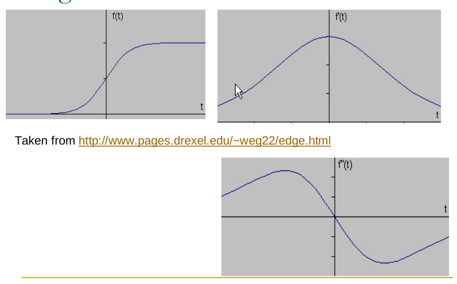
• Intuition (1D): Imagine a smoothed step edge. Its profile is like a ramp (sigmoid).
  • The first derivative is a bump (peak).
  • The second derivative (LoG in 1D) is positive on one side of the peak, negative on the other, and crosses zero exactly at the location of the peak of the first derivative. This peak corresponds to the point of maximum slope in the smoothed edge profile, which is considered the edge location.
• In 2D: Zero-crossings in the LoG image form closed contours corresponding to the boundaries of objects (at the scale defined by $\sigma$).
• Output: The output of the LoG edge detector is typically a binary image where pixels corresponding to zero-crossings are marked (e.g., value 1) and all other pixels are not (e.g., value 0).

Implementation Steps

1. Choose Sigma ($\sigma$): Select the standard deviation for the Gaussian. This determines the scale of edges to be detected. Larger $\sigma$ detects larger, smoother edges and provides more noise suppression. Smaller $\sigma$ detects finer details but is more sensitive to noise.
2. Generate LoG Kernel: Create a discrete approximation of the ${\nabla }^2{G}_{\sigma }(x,y)$ kernel (e.g., a $5\times 5$, $7\times 7$, or larger mask). The size depends on $\sigma$.
3. Convolution: Convolve the input image $I(x,y)$ with the discrete LoG kernel. Let the result be $R(x,y)$.
4. Detect Zero-Crossings: Scan the resulting image $R(x,y)$ to find locations where the value changes sign between adjacent pixels.
   • Common checks involve comparing $R(i,j)$ with its neighbors $R(i+1,j)$ and $R(i,j+1)$. A sign change indicates a zero-crossing between the pixels.
   • Often, a threshold is applied to the difference in values across the zero-crossing (or the local gradient magnitude) to avoid detecting spurious crossings caused by noise in flat regions. Only zero-crossings with a sufficiently large slope (magnitude difference) are kept.

Role of Sigma ($\sigma$)

• $\sigma$ acts as a scale parameter.
• It controls the degree of smoothing applied before edge detection.
• By varying $\sigma$, edges of different sizes or prominence can be detected (multi-scale edge detection).

Approximation: Difference of Gaussians (DoG)

• The LoG kernel (${\nabla }^2{G}_{\sigma }$) can be efficiently approximated by the Difference of Gaussians (DoG).
• This involves subtracting two Gaussian-smoothed versions of the image, obtained using slightly different standard deviations, ${\sigma }_1$ and ${\sigma }_2$ (typically ${\sigma }_2\approx 1.6{\sigma }_1$). $DoG(I)\approx (G_{{\sigma }_1}\ast I)-(G_{{\sigma }_2}\ast I)=(G_{{\sigma }_1}-G_{{\sigma }_2})\ast I$
• The shape of the $G_{{\sigma }_1}-G_{{\sigma }_2}$ kernel closely resembles the LoG kernel.
• Advantage: Gaussian smoothing can often be implemented very efficiently (e.g., using separable kernels or FFT). Computing two Gaussian smoothings and subtracting might be faster than direct convolution with a large LoG kernel.

Advantages of LoG/Marr-Hildreth

1. Good Localization: Zero-crossings accurately pinpoint edge locations in the smoothed image.
2. Scale Parameter: $\sigma$ allows tuning for specific edge scales and noise levels.
3. Noise Reduction: Initial Gaussian smoothing makes it less sensitive to noise than the raw Laplacian.
4. Closed Contours: The detected zero-crossings naturally form closed boundaries.

Disadvantages of LoG/Marr-Hildreth

1. Computational Cost: Convolution with larger LoG (or DoG) kernels can be computationally intensive.
2. Spurious Responses: Can still produce zero-crossings in textured regions or due to noise if thresholding is not adequate.
3. Scale Selection: The optimal $\sigma$ may vary across the image or be application-dependent.
4. Corner Detection: Being an isotropic (rotationally symmetric) operator, it might round off or poorly detect sharp corners where edges meet at acute angles.

---