SVM Classifier Short Notes

Binary Classification

Problem Definition

• Given: Training data consisting of $N$ pairs $({\mathbf{x}}_i,y_i)$ for $i=1,\dots ,N$.
  • ${\mathbf{x}}_i\in {\mathbb{R}}^d$ is the feature vector for the $i$-th data point (input).
  • $y_i\in \{-1,1\}$ is the class label for the $i$-th data point (output).
• Goal: Learn a classifier function $f(\mathbf{x})$ such that it can predict the class label for new, unseen data points.
• Desired Property: For the training data, the classifier should ideally satisfy: $$f({\mathbf{x}}_i)\{\begin{array}{ll}\ge 0& \text{if }{y}_i=+1\\ <0& \text{if }{y}_i=-1\end{array}$$
• Correct Classification Condition: This can be concisely written as $y_{i}f({\mathbf{x}}_i)>0$ for a correct classification. (Note: The boundary case $f({\mathbf{x}}_i)=0$ is sometimes included in the positive class, as shown in the slide definition).

---

Review of Linear Classifiers

Linear Separability

• Definition: A dataset is linearly separable if there exists a linear discriminant function (a line in 2D, a plane in 3D, a hyperplane in higher dimensions) that can perfectly separate the data points of the different classes.

Linear Classifiers: Definition and Form

• General Form: A linear classifier has the discriminant function: $f(\mathbf{x})={\mathbf{w}}^T\mathbf{x}+b$
  • $\mathbf{w}\in {\mathbb{R}}^d$: Weight vector.
  • $b\in \mathbb{R}$: Bias (or intercept).
  • $\mathbf{x}\in {\mathbb{R}}^d$: Input feature vector.
• Decision Boundary: The boundary between the classes is defined by the equation $f(\mathbf{x})=0$, which is: ${\mathbf{w}}^T\mathbf{x}+b=0$
• Geometric Interpretation:
  • In 2D: The decision boundary is a line.
    • $\mathbf{w}$ is the vector normal (perpendicular) to the line.
    • $b$ determines the offset of the line from the origin.
    • Points on one side of the line have $f(\mathbf{x})>0$, points on the other side have $f(\mathbf{x})<0$.
  • In 3D: The decision boundary is a plane. $\mathbf{w}$ is the normal vector to the plane.
  • In nD (n > 3): The decision boundary is a hyperplane. $\mathbf{w}$ is the normal vector to the hyperplane.
• Comparison with K-NN:
  • K-NN: Requires storing (carrying) the entire training dataset to make predictions.
  • Linear Classifier: Uses the training data only to learn the parameters $\mathbf{w}$ and $b$. After learning, the training data is discarded. Only $\mathbf{w}$ and $b$ are needed for classifying new data.

The Perceptron Classifier

• Goal: Given linearly separable data ${\mathbf{x}}_i$ with labels $y_i\in \{-1,1\}$, find a weight vector $\mathbf{w}$ and bias $b$ such that the discriminant function $f({\mathbf{x}}_i)={\mathbf{w}}^T{\mathbf{x}}_i+b$ correctly separates all data points, i.e., $y_i({\mathbf{w}}^T{\mathbf{x}}_i+b)>0$.
• Finding the Separating Hyperplane: The Perceptron Algorithm provides a method.

The Perceptron Algorithm

1. Homogeneous Coordinates (Optional but convenient):
   • Rewrite the classifier as $f({\mathbf{x}}_i)={\tilde{\mathbf{w}}}^T{\tilde{\mathbf{x}}}_i+w_0$, where $\tilde{\mathbf{w}}$ are the weights for the original features and $w_0$ is the bias $b$.
   • Define an augmented weight vector $\mathbf{w}=(\tilde{\mathbf{w}},w_0)$ and an augmented feature vector ${\mathbf{x}}_i=({\tilde{\mathbf{x}}}_i,1)$.
   • The classifier becomes $f({\mathbf{x}}_i)={\mathbf{w}}^T{\mathbf{x}}_i$.
   • Note: The slides use this notation implicitly. We will use $\mathbf{w}$ for the potentially augmented vector and ${\mathbf{x}}_i$ for the potentially augmented input.
2. Initialization: Initialize the weight vector $\mathbf{w}=0$. Set a learning rate $\alpha >0$ (often $\alpha =1$).
3. Cycle through Data: Iterate through the data points $({\mathbf{x}}_i,y_i)$ repeatedly.
4. Check for Misclassification: For the current point ${\mathbf{x}}_i$, calculate $f({\mathbf{x}}_i)={\mathbf{w}}^T{\mathbf{x}}_i$. The point is misclassified if $y_{i}f({\mathbf{x}}_i)\le 0$.
5. Update Rule: If ${\mathbf{x}}_i$ is misclassified: $\mathbf{w}\leftarrow \mathbf{w}+\alpha \cdot \text{sign}(f({\mathbf{x}}_i))\cdot {\mathbf{x}}_i$
   • Note on the update: The standard Perceptron update is often written as $\mathbf{w}\leftarrow \mathbf{w}+\alpha y_i{\mathbf{x}}_i$. If $y_{i}f({\mathbf{x}}_i)\le 0$, then $y_i$ and $f({\mathbf{x}}_i)$ have opposite signs (or $f({\mathbf{x}}_i)=0$). The term $\text{sign}(f({\mathbf{x}}_i))$ as used in the slide seems potentially incorrect or non-standard. Using $\mathbf{w}\leftarrow \mathbf{w}+\alpha y_i{\mathbf{x}}_i$ directly adjusts $\mathbf{w}$ in the direction that increases $f({\mathbf{x}}_i)$ if $y_i=+1$ and decreases $f({\mathbf{x}}_i)$ if $y_i=-1$. Sticking precisely to the slide: $\mathbf{w}\leftarrow \mathbf{w}+\alpha \cdot \text{sign}(f({\mathbf{x}}_i))\cdot {\mathbf{x}}_i$. (See Page 7 example which uses $w\leftarrow w-\alpha x_i$ when $f(x_i)<0$, implying $\text{sign}(f(x_i))=-1$ was used.)
6. Termination: Repeat steps 3-5 until no misclassifications occur during a full cycle through the data.

Perceptron Example (2D - Page 7)

• Illustrates the update rule.
• Before Update: Shows a data point ${\mathbf{x}}_i$ (blue circle, assume $y_i=+1$) misclassified by the current boundary defined by $\mathbf{w}$ (since it’s below the line, $f({\mathbf{x}}_i)<0$).
• Update: Since $f({\mathbf{x}}_i)<0$, $\text{sign}(f({\mathbf{x}}_i))=-1$. The update is $\mathbf{w}\leftarrow \mathbf{w}-\alpha {\mathbf{x}}_i$. This moves the weight vector $\mathbf{w}$ away from ${\mathbf{x}}_i$.
• After Update: Shows the new weight vector and the corresponding shifted decision boundary, which is now closer to classifying ${\mathbf{x}}_i$ correctly.
• Final Weights: After convergence, the final weight vector $\mathbf{w}$ can be expressed as a linear combination of the training data points: $\mathbf{w}={\sum }_{i=1}^N{\alpha }_i{\mathbf{x}}_i$, where ${\alpha }_i$ reflects how often point ${\mathbf{x}}_i$ contributed to an update.

Perceptron Properties

• Convergence Theorem: If the training data is linearly separable, the Perceptron algorithm is guaranteed to converge to a separating hyperplane in a finite number of steps.
• Convergence Speed: Convergence can be slow.
• Solution Quality: The algorithm finds any separating hyperplane, not necessarily the “best” one. The resulting separating line can be very close to the training data points.
• Generalization: A line close to the data points might not generalize well to new, unseen data. We would prefer a solution with a larger margin.

---

Support Vector Machine (SVM) Classifier

The Concept of Margin

• Problem: For linearly separable data, there can be infinitely many separating hyperplanes. Which one is the best?
• Idea: Choose the hyperplane that maximizes the margin.
• Margin: The margin is the distance between the separating hyperplane and the closest data point(s) from either class. The total width of the “empty” slab around the decision boundary is twice this distance.
• Maximum Margin Solution: The hyperplane that maximizes this margin. This solution is considered the most stable under perturbations of the input data points and often leads to better generalization.
• Support Vectors: The data points that lie exactly on the margin boundaries (closest to the separating hyperplane) are called support vectors. They “support” the hyperplane.

Geometric Intuition (Linearly Separable Case)

• 
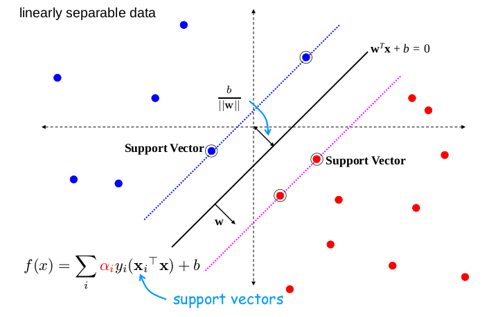
  • Decision Boundary: The solid line ${\mathbf{w}}^T\mathbf{x}+b=0$.
  • Margin Boundaries: Two dashed lines parallel to the decision boundary, defined by ${\mathbf{w}}^T\mathbf{x}+b=+1$ and ${\mathbf{w}}^T\mathbf{x}+b=-1$.
  • Margin Width: The perpendicular distance between the two margin boundaries is $\frac{2}{\Vert \mathbf{w}\Vert }$.
  • Support Vectors: The data points (circled) that lie exactly on the margin boundaries.
• Classifier Form: The final SVM classifier can be expressed as a sum involving only the support vectors: $f(\mathbf{x})={\sum }_{i\in \text{Support Vectors}}{\alpha }_i{y}_i({\mathbf{x}}_i^T\mathbf{x})+b$ (This form arises from the dual formulation, mentioned later).

Margin Calculation and Normalization (Sketch Derivation)

1. Scaling Freedom: The hyperplane ${\mathbf{w}}^T\mathbf{x}+b=0$ is the same as $c({\mathbf{w}}^T\mathbf{x}+b)=0$ for any constant $c\ne 0$. We can exploit this to choose a specific normalization for $\mathbf{w}$ and $b$.
2. Canonical Hyperplanes: Choose the scaling such that for the support vectors ${\mathbf{x}}_{+}$ (positive class) and ${\mathbf{x}}_{-}$ (negative class) closest to the hyperplane:
   • ${\mathbf{w}}^T{\mathbf{x}}_{+}+b=+1$
   • ${\mathbf{w}}^T{\mathbf{x}}_{-}+b=-1$ These define the margin boundaries.
3. Margin Calculation:
   • Consider the vector difference between support vectors on opposite margins: $({\mathbf{x}}_{+}-{\mathbf{x}}_{-})$.
   • The distance between the margin hyperplanes is the projection of this vector onto the normal vector $\frac{\mathbf{w}}{\Vert \mathbf{w}\Vert }$.
   • Margin Width = $\left|\frac{{\mathbf{w}}^T}{\Vert \mathbf{w}\Vert }({\mathbf{x}}_{+}-{\mathbf{x}}_{-})\right|$
   • Substitute ${\mathbf{w}}^T{\mathbf{x}}_{+}=1-b$ and ${\mathbf{w}}^T{\mathbf{x}}_{-}=-1-b$: Margin Width = $\left|\frac{(1-b)-(-1-b)}{\Vert \mathbf{w}\Vert }\right|=\left|\frac{1-b+1+b}{\Vert \mathbf{w}\Vert }\right|=\frac{2}{\Vert \mathbf{w}\Vert }$.

Optimization Problem (Hard Margin SVM)

• Goal: Maximize the margin width $\frac{2}{\Vert \mathbf{w}\Vert }$.

• Constraints: All data points must be correctly classified and lie on or outside their respective margin boundary. Using the canonical representation, this means:

  • ${\mathbf{w}}^T{\mathbf{x}}_i+b\ge +1$ for $y_i=+1$
  • ${\mathbf{w}}^T{\mathbf{x}}_i+b\le -1$ for $y_i=-1$
  • These can be combined into a single constraint: $y_i({\mathbf{w}}^T{\mathbf{x}}_i+b)\ge 1$ for all $i=1,\dots ,N$.

• Equivalent Optimization Problem: Maximizing $\frac{2}{\Vert \mathbf{w}\Vert }$ is equivalent to minimizing $\Vert \mathbf{w}\Vert$, which is equivalent to minimizing $\frac{1}{2}\Vert \mathbf{w}{\Vert }^2$ (the $\frac{1}{2}$ is often added for mathematical convenience in derivation, though the slide omits it). Primal Formulation (Hard Margin):

  $$\begin{gathered} \underset{\mathbf{w},b}{\min }\Vert \mathbf{w}{\Vert }^2 \\ \text{subject to}{y}_i({\mathbf{w}}^T{\mathbf{x}}_i+b)\ge 1,\text{for }i=1,\dots ,N \end{gathered}$$

  (Note: Slide 13 uses $\max \frac{2}{\Vert \mathbf{w}\Vert }$ and $\min \Vert \mathbf{w}{\Vert }^2$, both are valid formulations).

• Properties:

  • This is a Quadratic Programming (QP) problem (quadratic objective, linear constraints).
  • It has a unique minimum because the objective function is convex and the constraints define a convex feasible region.

Limitations of Hard Margin and Need for Soft Margin

• Problem 1: Strict Separability: The hard margin SVM requires the data to be perfectly linearly separable. It cannot handle data that is not linearly separable (as in page 3 bottom examples).
• Problem 2: Sensitivity to Outliers: Even if data is separable, a single outlier might force the margin to be very narrow, potentially leading to a less robust classifier (as hinted in page 14 top example).
• Trade-off: Sometimes, allowing a few points to be misclassified or lie within the margin might lead to a much larger margin and better overall generalization (as suggested in page 14 bottom example).

Soft Margin SVM: Slack Variables

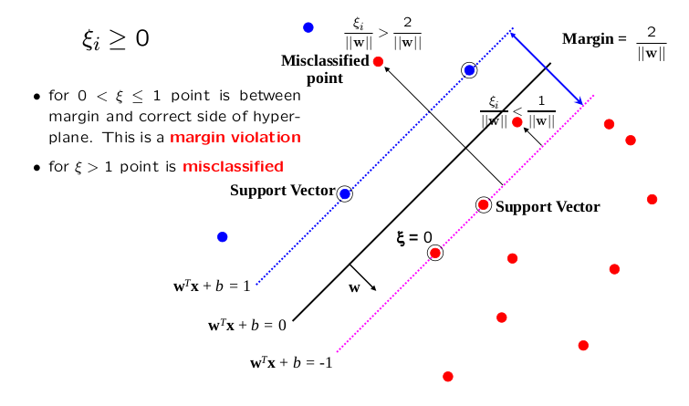
• Idea: Introduce slack variables, denoted by ${\xi }_i$ (Greek letter xi), for each data point ${\mathbf{x}}_i$.
• Purpose: Allow individual points to violate the margin constraint $y_i({\mathbf{w}}^T{\mathbf{x}}_i+b)\ge 1$.
• Modified Constraint: $y_i({\mathbf{w}}^T{\mathbf{x}}_i+b)\ge 1-{\xi }_i$
• Slack Variable Constraint: We require ${\xi }_i\ge 0$.
• Interpretation of ${\xi }_i$ (Page 15):
  • ${\xi }_i=0$: Point ${\mathbf{x}}_i$ is correctly classified and is on or outside the margin boundary (satisfies the hard margin constraint).
  • $0<{\xi }_i\le 1$: Point ${\mathbf{x}}_i$ is correctly classified ($y_{i}f({\mathbf{x}}_i)>0$) but lies inside the margin ($y_{i}f({\mathbf{x}}_i)<1$). This is a margin violation.
  • ${\xi }_i>1$: Point ${\mathbf{x}}_i$ is misclassified ($y_{i}f({\mathbf{x}}_i)<0$).
• Penalty: We want to minimize the total amount of slack introduced.

Optimization Problem (Soft Margin SVM)

• Objective: Minimize a combination of the classifier complexity (related to margin width) and the total slack. Primal Formulation (Soft Margin):

  $$\underset{\mathbf{w},b,\mathbf{\xi }}{\min }\Vert \mathbf{w}{\Vert }^2+C\sum _{i=1}^N{\xi }_i$$

  $\text{subject to}$ $$\quad y_i (\mathbf{w}^T \mathbf{x}_i + b) \ge 1 - \xi_i, \quad \text{for } i = 1, \dots, N $$$$ \quad \xi_i \ge 0, \quad \text{for } i = 1, \dots, N

  - $\boldsymbol{\xi} = (\xi_1, \dots, \xi_N)$ is the vector of slack variables. - $C \ge 0$ is the **regularization parameter**.

• Role of Regularization Parameter $C$:

  • Controls the trade-off between maximizing the margin (minimizing $\Vert \mathbf{w}{\Vert }^2$) and minimizing the classification/margin errors (minimizing $\sum {\xi }_i$).
  • Small $C$: Lower penalty on slack variables (${\xi }_i$). Allows more points to violate the margin (larger ${\xi }_i$) in favor of achieving a wider margin (smaller $\Vert \mathbf{w}{\Vert }^2$). Can lead to simpler models, potentially underfitting if too small.
  • Large $C$: Higher penalty on slack variables. Forces the optimizer to minimize margin violations. Behaves more like the hard margin SVM. Can lead to narrower margins and potentially overfitting if too large.
  • $C=\infty$: Corresponds to the hard margin SVM (no slack allowed).

• Properties:

  • Still a Quadratic Programming problem.
  • Has a unique minimum.
  • $C$ is a hyperparameter that needs to be chosen (e.g., via cross-validation).

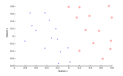
Examples of Varying C (Pages 17-19)

• Data: 2D data that is linearly separable but requires a narrow margin for perfect separation (Page 17).
• Case 1: $C=\infty$ (Hard Margin - Page 18)
  • Finds the separating hyperplane with the largest margin while correctly classifying all points.
  • Result: Margin = 0.0966, Training error = 0.00%, 3 Support Vectors. The margin is very narrow.
• Case 2: $C=10$ (Soft Margin - Page 19)
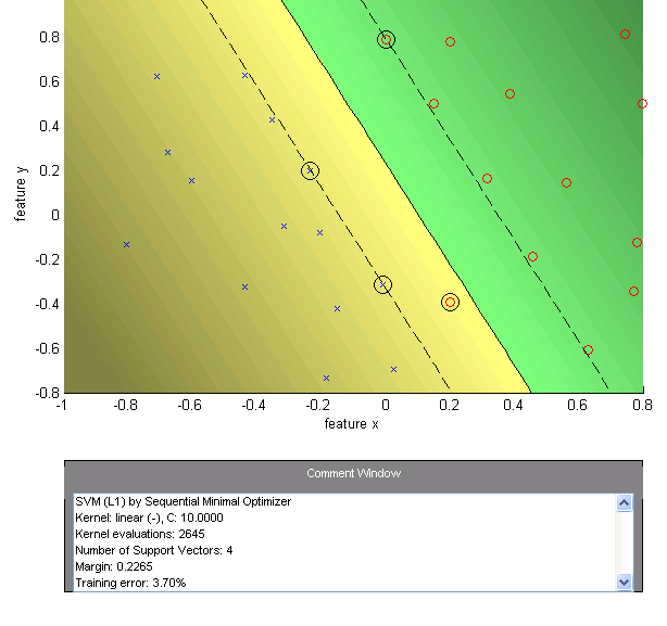
  • Allows some margin violation to potentially achieve a wider margin.
  • Result: Margin = 0.2265, Training error = 3.70% (one point is likely inside the margin or misclassified), 4 Support Vectors. The margin is significantly wider.

---

Application: Pedestrian Detection in Computer Vision

Objective

• Detect (localize) standing humans in images.

Approach: Sliding Window Classifier

1. Define a window of a fixed size.
2. Slide this window across the image at different positions and scales.
3. For each window, classify whether it contains the object of interest (a pedestrian) or not.
4. This reduces object detection to a binary classification problem.