Shape Representation

6.1 Introduction

A shape is a binary image. Mathematically, it is defined as:

$f(x,y)=\{\begin{array}{ll}1& \text{if }(x,y)\in D\\ 0& \text{otherwise}\end{array}$ (6.1)

where $D$ is the domain or area of the binary image.

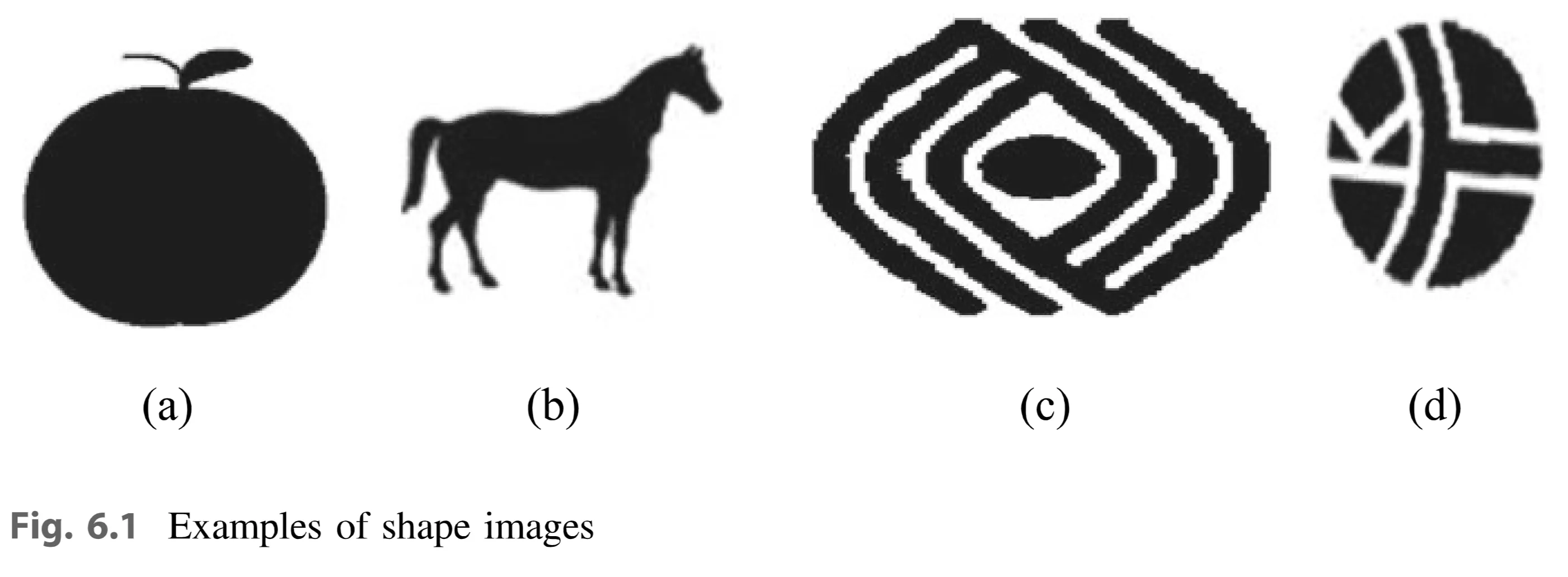
good for shap, p.2 Most objects in the world can be identified by their shapes (e.g., fruits, trees, leaves, buildings, furniture, birds, fishes). A shape can be defined by its boundary/contour (like Fig. 6.1a and b, which are not reproduced here, but described as shapes with a contour) or by its interior content (like Fig. 6.1c and d, described as shapes with interior content).

There are various shape methods, generally grouped into:

• Contour-based methods: Focus on the outline or boundary of the shape.
• Region-based methods: Consider the entire area occupied by the shape.
• Perceptual shape descriptors: use to capture both contour and region feature.

Shape descriptor design (as suggested by MPEG-7) typically aims for:

• Good retrieval accuracy
• Compact features
• General application
• Low computation complexity
• Robust retrieval performance (affine invariance and noise resistance)
• Hierarchically coarse to fine representation.

Shape description is challenging due to difficulties in defining perceptual features, measuring similarity, and dealing with noise, defects, distortion, and occlusion.

6.2 Perceptual Shape Descriptors

These descriptors are based on human perception and can be combined for a more robust representation.

6.2.1 Circularity and Compactness

Circularity indicates how close a shape is to a circle, reflecting its compactness. It’s defined as the ratio of the shape’s area ($A_s$) to the area of a circle ($A_c$) with the same perimeter:

$C=\frac{A_s}{A_c}$ (6.2)

If $p$ is the perimeter of the shape, the area of the circle with the same perimeter is:

$A_c=\frac{p^2}{4\pi }$ (6.3)

Therefore:

$C=\frac{4\pi A_s}{p^2}$ (6.4)

Since $4\pi$ is a constant, circularity can be simplified as:

$C=\frac{A_s}{p^2}$ (6.5)

A perfect circle has a circularity of 1.

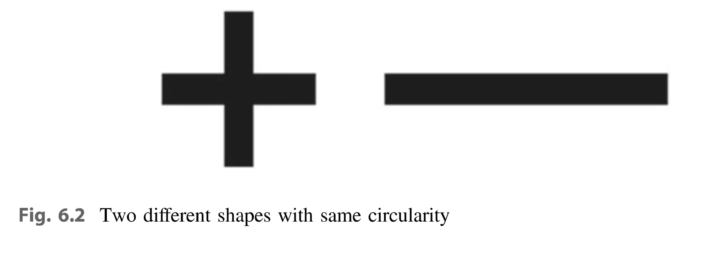
good for shap, p.3 Limitations: This definition can be misleading. Different-looking shapes (e.g., Fig. 6.2, a plus sign and a horizontal line) can have the same circularity. It is also sensitive to noise and irregularities.

A more robust circularity descriptor is defined as:

$C=\frac{{\sigma }_R}{{\mu }_R}$ (6.6)

where:

• ${\mu }_R$ is the mean of the radial distance from the shape’s centroid to its boundary points.
• ${\sigma }_R$ is the standard deviation of the radial distance from the centroid to the boundary points.

6.2.2 Eccentricity and Elongation

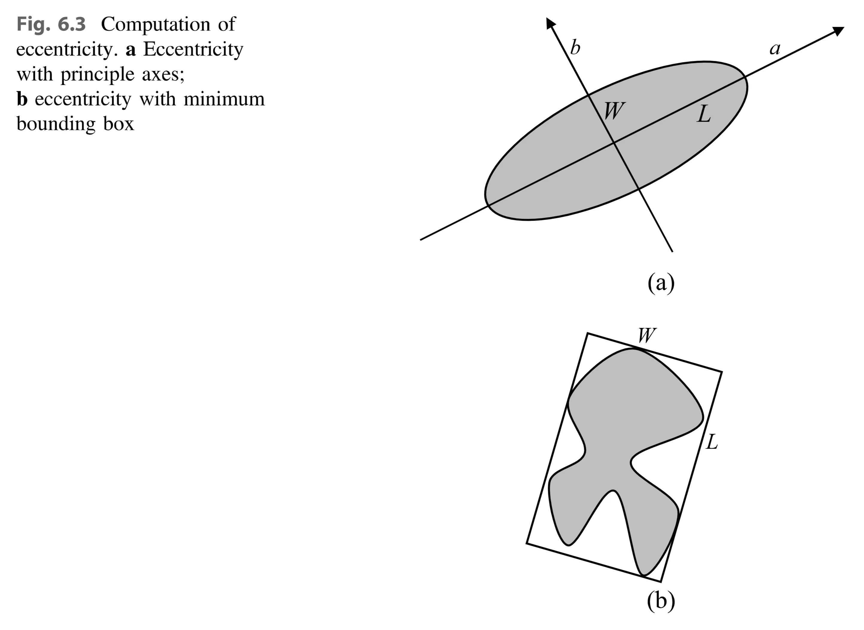
Eccentricity is the ratio of the length of the longest chord of the shape ($L$) to the length of the longest chord perpendicular to it ($W$). It can be calculated using: good for shap, p.4

• Principal axis method: (Fig. 6.3a - depicts an ellipse with its major axis ‘a’, minor axis ‘b’, longest chord ‘L’ along the major axis, and chord ‘W’ perpendicular to ‘L’)
• Minimum bounding box method: (Fig. 6.3b - shows an irregular shape enclosed in a rectangle. ‘L’ represents the longer side of the rectangle, and ‘W’ represents the shorter side.)

$E=\frac{L}{W}$ (6.7)

Eccentricity indicates elongation. A larger eccentricity means a more elongated shape.

Elongation is defined as:

$El=1-\frac{W}{L}$ (6.8)

• $0\le El\le 1$
• Circle, square, or symmetric shapes have Elongation = 0.
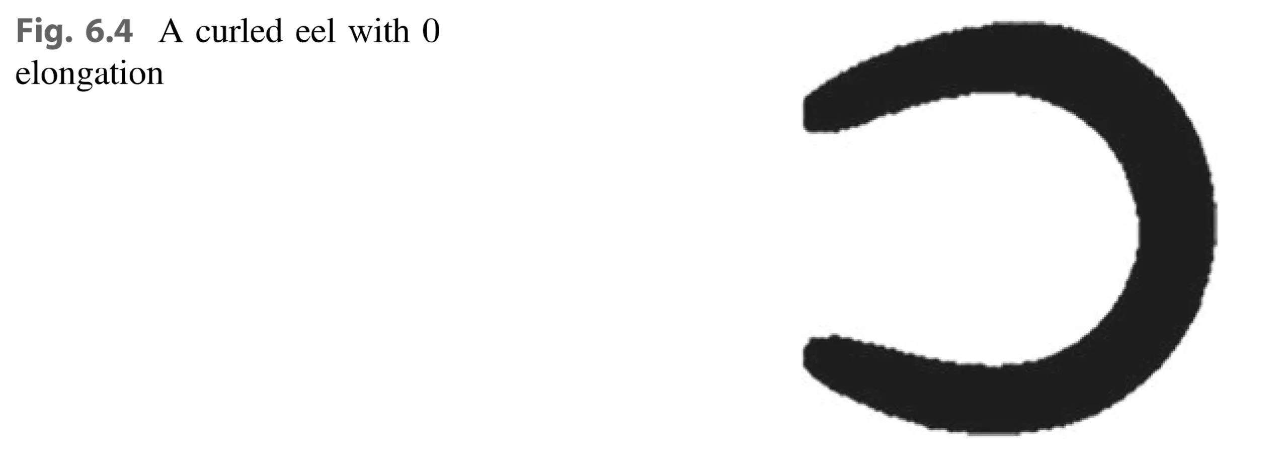
• Elongated objects (eels, poles, roads) have Elongation close to 1. good for shap, p.5 Limitation: Elongation can fail for bent, elongated shapes (e.g., a curled eel - Fig. 6.4 - would have a low elongation).

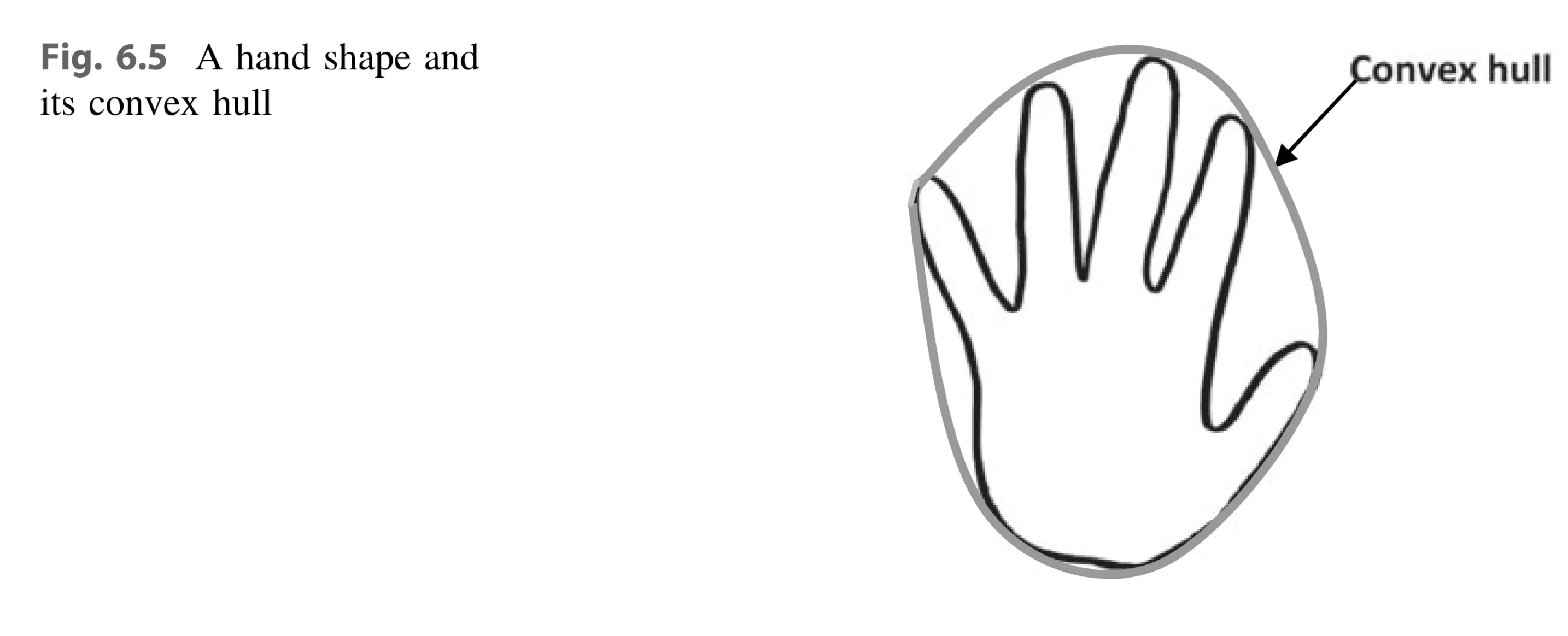
6.2.3 Convexity and Solidarity

• Convex Region: A region is convex if, for any two points within the region, the entire line segment connecting them is also inside the region.
• Convex Hull: The smallest convex region that includes the shape (Fig. 6.5 - shows a hand shape and its enclosing convex hull). good for shap, p.5

Convexity is the ratio of the perimeter of the convex hull ($P_h$) to the perimeter of the shape ($P_s$):

$\text{Convexity}=\frac{P_h}{P_s}$ (6.9)

Solidarity is the ratio of the area of the shape ($A_s$) to the area of its convex hull ($A_h$):

$\text{Solidarity}=\frac{A_s}{A_h}$ (6.10)

• Convex shapes: Convexity and Solidarity = 1.
• Non-convex shapes: Convexity and Solidarity < 1.

6.2.4 Euler Number

Topology studies properties unaffected by deformation (e.g., rubber-sheet distortion). The number of holes in a shape remains constant under deformation.

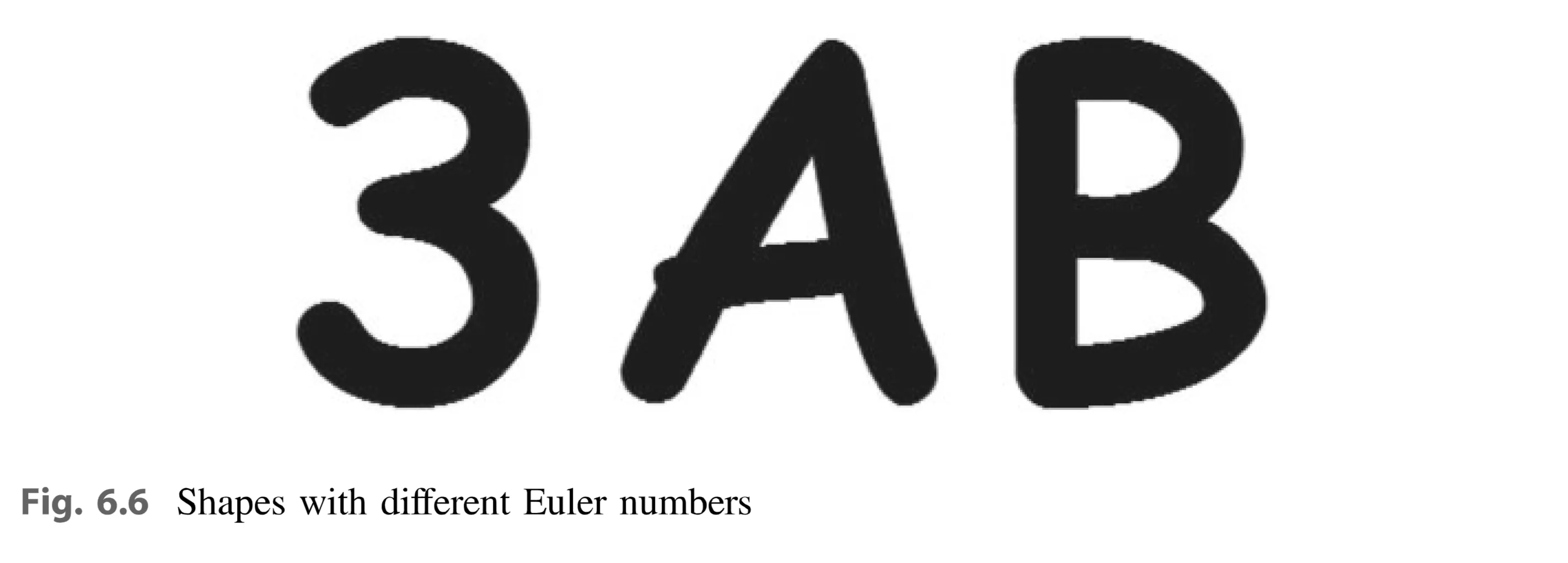
Euler Number (En): The difference between the number of connected components ($C$) and the number of holes ($H$).

$En=C-H$ (6.11)

A smaller Euler number indicates more holes. (Fig. 6.6 shows the number 3, and letters A and B. Their Euler numbers are 1, 0, and -1, respectively). good for shap, p.6

Hole Area Ratio (HAR):

$HAR=\frac{A_h}{A_s}$ (6.12)

where:

• $A_h$ is the total area of holes.
• $A_s$ is the area of the shape.

6.2.5 Bending Energy

Bending Energy (BE) is defined as:

$BE=\frac{1}{N}{\sum }_{t=0}^{N}K(t{)}^2$ (6.13)

and

$K(t)=\frac{(\dot{x}(t)\ddot{y}(t)-\ddot{x}(t)\dot{y}(t))}{({\dot{x}}^2(t)+{\dot{y}}^2(t){)}^{3/2}}$ (6.14)

where:

• $K(t)$ is the curvature function.
• $N$ is the number of points on a contour.
• $\dot{x}(t)$ and $\dot{y}(t)$ are the first derivatives of x(t) and y(t).
• $\ddot{x}(t)$ and $\ddot{y}(t)$ are the second derivatives of x(t) and y(t).

The shape boundary is usually Gaussian-smoothed before BE calculation. A circle has the minimum bending energy.

Advantages of Perceptual Descriptors: They have semantic meaning.

Disadvantages of Perceptual Descriptors: They can be sensitive (as seen with circularity and eccentricity). A single descriptor is often insufficient. They’re often used as filters.

6.3 Contour-Based Shape Methods

These methods use only shape boundary information. Two main approaches:

1. Continuous (Global) Approach: Doesn’t divide the shape into subparts. A multidimensional feature vector derived from the entire boundary describes the shape.
2. Discrete (Structural) Approach: Breaks the boundary into segments (primitives) based on a criterion. Representation is a string or graph.

6.3.1 Shape Signatures

The first step is to obtain a 1D function (shape signature) from the boundary points. Many types exist:

• Complex coordinates
• Polar coordinates
• Central distance
• Tangent angle
• Cumulative angle
• Curvature
• Area
• Chord length

In general, a shape signature $u(t)$ is any 1D function representing 2D areas or boundaries, capturing perceptual features and uniquely describing the shape. Assume boundary coordinates $(x(t),y(t)),t=0,1,...,N-1$ are extracted, and $t$ usually represents arc length. Preprocessing typically involves denoising/smoothing and contour tracing.

6.3.1.4 Curvature Signature

Curvature is an important boundary feature, defined as:

$\kappa (t)=\frac{d\theta }{dt}$ (6.20a)

$=\frac{x^{\prime }{y}^{\prime \prime }-y^{\prime }{x}^{\prime \prime }}{(x^{\prime 2}+y^{\prime 2}{)}^{3/2}}$ (6.20b)

$=\frac{\frac{d^{2}y}{d{x}^2}}{(1+(\frac{dy}{dx}{)}^2{)}^{3/2}}$ (6.20c)

• A perfect circle has a constant $k(t)$.
• $k(t)$ is often zero and jumps at discontinuities in $\theta (t)$.
• Requires smoothing before extraction (Fig. 6.10 shows curvature of the tree from Fig. 6.7, with and without smoothing.)
• Invariant to translation.
• Rotation causes a circular shift.
• Invariant to scaling if shapes are normalized to the same number of points.

6.3.3 Boundary Moments

Moments reduce the dimension of a boundary representation. The $r$th moment $m_r$ and central moment ${\mu }_r$ of shape signature $z(i)$ are:

$m_r=\frac{1}{N}{\sum }_{i=1}^N[z(i){]}^r$ and ${\mu }_r=\frac{1}{N}{\sum }_{i=1}^N[z(i)-m_1{]}^r$ (6.22)

Normalized moments $m_r$ and ${\mu }_r$ are invariant to translation, rotation and scaling.

Moments can also be computed from the boundary histogram $p(v_i)$ of quantized $z(i)$:

${\mu }_r={\sum }_{i=1}^K(v_i-m{)}^{r}p(v_i)$ and $m={\sum }_{i=1}^K{v}_{i}p(v_i)$ (6.23)

• Simple to compute, more robust than shape signatures.
• Only low-order moments have physical meaning.
  • $F_1=({\mu }_2{)}^{1/2}/m_1$ (variance)
  • $F_2={\mu }_3/({\mu }_2{)}^{3/2}$ (skewness)
  • $F_3={\mu }_4/({\mu }_2{)}^2$ (kurtosis)

6.3.6 Fourier Descriptor

For 1D signature function $f(x)$, the discrete Fourier transform is:

$a_n=\frac{1}{N}{\sum }_{t=0}^{N-1}f(x)\exp (-j2\pi nx/N),n=0,1,...,N-1$ (6.26)

$\{a_n\}$ is a representation of the shape. Magnitudes $|a_n|$ are invariant to rotation and starting point.

• Translation Invariance: Normalize to the centroid or subtract the mean.
• Scale Invariance: Normalize by the DC component $a_0$:

$|b_n|=|a_n|/a_0,n=1,2,...,N-1$ (6.27)

$\{|b_n|,1<n<N-1\}$ is used as the shape descriptor (FD).

• Efficient to compute (FFT).
• Coarse to fine representation.
• FDs have physical meaning.
• Simple matching (city block or Euclidean distance).
• Robust.

6.3.9 Polygon Decomposition

Captures overall shape, discards minor variations.

• Merging: Add pixels to a line segment if the deviation is small. Total squared error is used. (Fig. 6.18 illustrates this).
• Splitting: Draw a line from start to end, compute perpendicular distances. Break into segments if the distance exceeds a threshold. (Fig. 6.19 shows polygon approximation by splitting.)

Segments are primitives (described by length, angle). Matching involves shift and best match (feature-by-feature, then model-by-model).

6.3.9.1 Chain Code Representation

Describes an object by a sequence of unit-size line segments with given orientations (4-connectivity or 8-connectivity) (Fig. 6.20 shows chain code in 8-connectivity and 4-connectivity).

• Invariant to translation.
• Rotation invariance: Find the pixel resulting in the minimum integer number.
• Matching: chain code histogram.
• Can be used to create polygon of a shape.

6.3.9.2 Smooth Curve Decomposition

Segment into boundary segments using curvature threshold. Smooth with Gaussian filter, then segment at points where curvature exceeds the threshold (Fig. 6.21 shows a horse shape segmented this way).

Primitives: maximum curvature and orientation. Matching: weighted Euclidean distance.

6.3.9.3 Discussions

Advantage of structural approach is to handle occlusion problem. But, suffer from ambiguity of primitives.

6.4 Region-Based Shape Feature Extraction

All pixels within a shape region are considered.

6.4.1 Geometric Moments

Projections of a function onto a polynomial basis. Geometric moment of order $(p+q)$ of function $f(x,y)$:

$M_{pq}={\int }_{-\infty }^{\infty }{\int }_{-\infty }^{\infty }{x}^p{y}^{q}f(x,y)dxdy,p,q=0,1,2,...$ (6.30)

• $Mass=M_{00}$ (6.31)
• $\text{Centroid}=\{\bar{x}=\frac{M_{10}}{M_{00}},\bar{y}=\frac{M_{01}}{M_{00}}\}$ (6.32)

Central moments of order $p+q$:

${\mu }_{pq}={\sum }_x{\sum }_y(x-\bar{x}{)}^p(y-\bar{y}{)}^{q}f(x,y)p,q=0,1,2,...$ (6.33)

Normalized central moments ${\mu }_{pq}/{\mu }_{00}$ are invariant to translation and scaling.

• $(m10/m00,m01/m00)$: center of gravity.
• $m_{20}$ and $m_{02}$: moments of inertia.
• ${\mu }_{10}/{\mu }_{00}$ and ${\mu }_{01}/{\mu }_{00}$: horizontal and vertical mean.
• ${\mu }_{20}/{\mu }_{00}$ and ${\mu }_{02}/{\mu }_{00}$: horizontal and vertical variance.
• ${\mu }_{11}$: covariance.
• ${\mu }_{30}/{\mu }_{00}$ and ${\mu }_{03}/{\mu }_{00}$: horizontal and vertical skewness.
• ${\mu }_{40}/{\mu }_{00}$ and ${\mu }_{04}/{\mu }_{00}$: horizontal and vertical kurtosis.

Not rotation invariant. Hu’s seven moment invariants (up to order three):

${\Phi }_1={\eta }_{20}+{\eta }_{02}$ ${\Phi }_2=({\eta }_{20}-{\eta }_{02}{)}^2+4({\eta }_{11}{)}^2$ ${\Phi }_3=({\eta }_{30}-3{\eta }_{12}{)}^2+(3{\eta }_{21}-{\eta }_{03}{)}^2$ ${\Phi }_4=({\eta }_{30}+{\eta }_{12}{)}^2+({\eta }_{21}+{\eta }_{03}{)}^2$ ${\Phi }_5=({\eta }_{30}-3{\eta }_{12})({\eta }_{30}+{\eta }_{12})[({\eta }_{30}+{\eta }_{12}{)}^2-3({\eta }_{21}+{\eta }_{03}{)}^2]+(3{\eta }_{21}-{\eta }_{03})({\eta }_{21}+{\eta }_{03})[3({\eta }_{30}+{\eta }_{12}{)}^2-({\eta }_{21}+{\eta }_{03}{)}^2]$ ${\Phi }_6=({\eta }_{20}-{\eta }_{02})[({\eta }_{30}+{\eta }_{12}{)}^2-({\eta }_{21}+{\eta }_{03}{)}^2]+4{\eta }_{11}({\eta }_{30}+{\eta }_{12})({\eta }_{21}+{\eta }_{03})$ ${\Phi }_7=(3{\eta }_{21}-{\eta }_{03})({\eta }_{30}+{\eta }_{12})[({\eta }_{30}+{\eta }_{12}{)}^2-3({\eta }_{21}+{\eta }_{03}{)}^2]+(3{\eta }_{12}-{\eta }_{30})({\eta }_{21}+{\eta }_{03})[3({\eta }_{30}+{\eta }_{12}{)}^2-({\eta }_{21}+{\eta }_{03}{)}^2]$ (6.34)

where ${\eta }_{pq}={\mu }_{pq}/({\mu }_{00}{)}^{\gamma }$ and $\gamma =1+(p+q)/2$ for $p+q=2,3,...$.

6.4.2 Complex Moments

Addresses rotation invariance using complex moments and polar sampling.

$C_{pq}={\int }_{-\infty }^{\infty }{\int }_{-\infty }^{\infty }(x+jy{)}^p(x-jy{)}^{q}f(x,y)dxdy$ (6.35)

where $j=\sqrt{-1}$.

Zernike Moments: Derived from Zernike polynomials:

$V_{nm}(x,y)=V_{nm}(\rho \cos \theta ,\rho \sin \theta )=R_{nm}(\rho )\exp (jm\theta )$ (6.36)

where

$R_{nm}(\rho )={\sum }_{s=0}^{(n-|m|)/2}(-1{)}^s\frac{(n-s)!}{s!(\frac{n+|m|}{2}-s)!(\frac{n-|m|}{2}-s)!}{\rho }^{n-2s}$ (6.37)

• $\rho$ is the radius.
• $\theta$ is the angle.

Shape is normalized to a unit disk. Examples of Zernike polynomials:

• $R_{00}(\rho )=1$
• $R_{11}(\rho )=\rho$
• $R_{20}(\rho )=2{\rho }^2-1$
• $R_{22}(\rho )={\rho }^2$
• $R_{31}(\rho )=3{\rho }^3-2\rho$
• $R_{33}(\rho )={\rho }^3$

(Fig 6.22. shows first 10 real Zernike polynomials). Complex Zernike moments:

$A_{nm}=\frac{n+1}{\pi }{\sum }_x{\sum }_{y}f(x,y)V_{nm}^{\ast }(x,y),x^2+y^2\le 1$ (6.38)

or

$A_{nm}=\frac{n+1}{\pi }{\sum }_{\rho }{\sum }_{\theta }f(\rho \cos \theta ,\rho \sin \theta )R_{nm}(\rho )\exp (jm\theta ),\rho \le 1$ (6.39)

Angular Radial Transformation (ART) (used by MPEG-7):

$AR{T}_{nm}=\frac{1}{2\pi }{\sum }_{\rho }{\sum }_{\theta }f(\rho \cos \theta ,\rho \sin \theta )V_{nm}(\rho ,\theta ),\rho \le 1$ (6.40)

where $V_{nm}$ is the ART basis function:

$V_{nm}=R_n(\rho )\exp (jm\theta )$ (6.41)

and $R_n(\rho )$ is the radial basis function:

$R_n(\rho )=\{\begin{array}{ll}1& \text{if }n=0\\ 2\cos (n\pi \rho )& \text{if }n\ne 0\end{array}$ (6.42)

(Table 6.1 lists Zernike moments up to order 10. Fig 6.23 shows first 36 Zernike moments and Fig.6.24. shows the real parts of the first 36 ART basis function).

• Invariant to rotation.
• More robust (captures spatial information).
• Minimum information redundancy.
• Computationally expensive.
• Unit disk normalization affects the accuracy.

6.4.3 Generic Fourier Descriptor

Combines advantages of complex moments and Fourier transform.

1. Transform shape into a rectangular polar image (sides $r$ and $\theta$). (Fig 6.25 shows polar raster transformation.
2. Apply 2D Fourier transform.
3. Use normalized Fourier coefficients as the descriptor. Centroid: $x_c=\frac{1}{M}{\sum }_{x=0}^{N-1}x$ $y_c=\frac{1}{N}{\sum }_{y=0}^{M-1}y$ (6.43)

$r=\sqrt{(x-x_c{)}^2+(y-y_c{)}^2}$, $\theta =arctan\frac{y-y_c}{x-x_c}$ (6.44)

Polar Fourier Transform (PFT):

$PF(\rho ,\theta )={\sum }_r{\sum }_{\theta }f(r,\theta )\exp \left[j2\pi \left(\frac{r}{R}\rho +\frac{\theta }{T}\right)\right]$ (6.45)

Generic Fourier Descriptor(GFD): $GFD=\left\{\frac{|PF(0,0)|}{area},\frac{|PF(0,1)|}{|PF(0,0)|},...,\frac{|PF(0,n)|}{|PF(0,0)|},...,\frac{|PF(m,0)|}{|PF(0,0)|},...,\frac{|PF(m,n)|}{|PF(0,0)|}\right\}$ (6.46)

• Captures shape information with fewer coefficients.
• Simpler and more efficient compared with ZMD.
• (Fig.6.26 shows an example of PFT on two shape images).

6.4.4 Shape Matrix

Binarize the shape within a bounding box.

1. Square centered at the center of gravity $G$.
2. Side length = $2L$, where $L=GM$ (maximum distance from $G$ to a boundary point $M$).
3. Normalize squares and align with line $L$.
4. Divide into $N\times N$ blocks $b_{ij}$.

Shape matrix $SM=[c_{ij}]$:

$c_{ij}=\{\begin{array}{ll}1& \text{if }A(S\cap b_{ij})>A(b_{ij})/2\\ 0& \end{array}$ (6.47)

where $A()$ is the area function. (Fig. 6 where $A()$ is the area function. (Fig. 6.27 shows a shape and its shape matrix).

• Invariant to translation, scale, and rotation.

Similarity of two shape matrices $A=[a_{ij}]$ and $B=[b_{ij}]$:

$d(A,B)=1-\frac{1}{N^2}{\sum }_{i=0}^N{\sum }_{j=0}^N|a_{ij}-b_{ij}|$ (6.48)

• Sensitive to boundary noise.
• Multiple guesses of longest radii are needed.

Polar Shape Matrix: More robust (uses a polar grid) (Fig 6.28 shows polar sampling of shape and its polar shape matrix). Rotation causes a horizontal shift.

6.4.5 Shape Profiles

6.4.5.1 Shape Projections

Projections of the shape onto x-axis and y-axis.

• Vertical Profile: $P_v(x)={\sum }_{y_{min}}^{y_{max}}f(x,y)$
• Horizontal Profile: $P_h(y)={\sum }_{x_{min}}^{x_{max}}f(x,y)$ (6.49)

(Fig. 6.29 shows a shape with its vertical and horizontal profiles.)

Unique to each type of object.

Polar shape profiles: Count pixels at each angle and radius.

6.4.5.2 Radon Transform

Multiple profiles from different directions $\theta$.

$R(\rho ,\theta )={\int }_{-\infty }^{\infty }{\int }_{-\infty }^{\infty }f(x,y)\delta (x\cos \theta +y\sin \theta -\rho )dxdy$ (6.50)

where:

• $\rho =x\cos \theta +y\sin \theta$ is the line.

• $\theta$ and $\rho$ are the angle and distance of the line.

• $\delta (x)$ is the Dirac delta function:

  • $\delta (x-a)=0$ for $x\ne a$ (6.51)
  • ${\int }_{-\infty }^{\infty }f(x)\delta (x-a)dx=f(a)$ (6.52)

(Fig. 6.30 illustrates a shape profile.)

(Fig. 6.31 shows profiles of a hammer at 90° and 8°.)

(Fig. 6.32 shows the Radon transform spectrum of the hammer.)

(Fig. 6.33 shows a dog shape and its Radon transform spectrum.)

A histogram or GFD can be computed from the Radon spectrum.

6.4.6 Discussions

Region based method use all pixels of shape, which makes them more robust than contour-based methods.

6.4.7 Convex Hull

• Convex Region: For any two points $x_1,x_2\in R$, the line segment $x_1{x}_2$ is inside $R$.
• Convex Hull: Smallest convex region $H$ such that $R\subset H$.
• Convex Deficiency ($D$): $H-R$.

Methods: morphological methods, polygon approximation.

Shape boundaries are often irregular. Smooth the boundary first.

Convex hull features can be extracted in a single process or recursively (concavity tree). (Fig. 6.34 shows the convex hull and concavity tree of an apple.)

Matching: string matching or graph matching. Smooth the boundary before extraction.

6.4.8 Medial Axis

Skeleton: A connected set of medial lines along the limbs of a figure. Eliminates redundant information, retains topology.

Medial Axis Transform (MAT): Locus of centers of maximal disks or bi-tangent circles that fit entirely within the shape (Fig. 6.35 shows medial axis computation.)

Decompose the skeleton into segments. Matching: graph matching.

• Sensitive to boundary noise.
• Smooth the contour first.

Medial axis from scale space: core.

Alternative: distance transform, ridge detection, linking (Fig. 6.36. shows a horse shape and its skeleton computed from distance map).

Region structural methods are useful for partial matching, but have complex computation and matching.

6.5 Summary

• Perceptual Descriptors: Intuitive, but not powerful enough alone. Used as filters.
• Contour Shape Descriptors: More sensitive to noise than region-based methods.
• Region-Based Methods: More robust (use all information within the region).

MPEG-7 principles: good retrieval accuracy, compact features, general application, low computation complexity, robust retrieval, hierarchical representation. FD, GFD, ZMD are desirable.

Choice of techniques depends on the application.

6.6 Exercises

5. Circularity/Compactness: Use boundary tracing and area code from the provided links to calculate circularity/compactness.

6. Elongation: Use provided Matlab code to extract the bounding box and calculate elongation.

7. Radon Transform: Use provided Matlab code to compute the Radon transform.

8. Radon Spectrum Statistics: Compute mean, standard deviation, and histogram of the Radon spectrum.

9. Comparison: Compare features from Radon spectra with those from Exercises 1 and 2.